In Faster Data Association with Max-Sum Loopy Belief Propagation (MASDA) I derived MASDA for the tracking problem: associate measurements with objects, allowing for clutter and misdetection. Stereo matching has the same structure, so this post applies MASDA there and measures what it gains.
Stereo is convenient for this. The one-to-one constraint is physically real, since a surface point projects once into each image. Ground truth is obtainable, so I can ask whether a match is correct rather than whether it looks plausible. And there is a strong baseline: the exact linear assignment problem, solved by Jonker-Volgenant.
Results, briefly:
- MASDA reaches the exact LAP optimum on all five test problems, three synthetic and two real.
- Against mutual nearest-neighbour with a ratio test, it finds 3.27× more correct matches on ambiguous texture, and 1-7% more where descriptors discriminate.
- Precision collapses for every method on ambiguous texture, including the exact solver. Uniqueness is real information but it is not sufficient information.
- An ordering factor folds into the same closed form for one clamped scalar per conflicting edge. On eight real scenes it cuts crossings by a third and returns about 1% more correct matches. On my synthetic scenes it looked useless or harmful, which says more about synthetic scenes than about ordering.
- The speed advantage depends entirely on representation. A dense implementation is slower than scipy’s Jonker-Volgenant; the same algorithm on an edge list is 157-230× faster.
- On real pairs the detector, not the matcher, is the binding constraint: only half the left keypoints have a right-image keypoint anywhere near their true correspondence, which caps recall before matching starts.
The synthetic half runs from one script with no input images, so the disparity is known exactly. The real half uses Middlebury’s Teddy and Cones, which ship quarter-pixel ground truth.
1. Stereo as a data association problem
In tracking, measurements \(i \in \{1 \dots m\}\) are associated with objects \(j \in \{1 \dots n\}\), at most one each way, with the option of calling a measurement clutter or an object misdetected.
For stereo, substitute the nouns. Keypoints in the left image are measurements, keypoints in the right image are objects. At most one association each way, because one surface point produces one projection per image. A left keypoint whose surface is occluded in the right view has no partner at all, which is clutter (\(\lambda\)). A right keypoint whose partner the left detector missed is a misdetection (\(\gamma\)).
Occlusion is not a small correction here. In the scene below, 30% of left keypoints have no attainable match, either because the surface is hidden or because the corresponding right keypoint was never detected. A formulation that assumes every keypoint is matchable is wrong a third of the time.
What stereo adds is geometry. The pair is rectified, so correspondences lie on the same image row and disparity \(d = x_L - x_R\) is positive and bounded. That makes the association graph very sparse, which turns out to matter a lot (section 6).
1.1 Factor graph
Same as the tracking case: binary association variables \(c_{ij}\), clutter indicators \(e_i\), misdetection indicators \(\delta_j\), similarity factors \(S_{ij}\), clutter factors \(\Lambda_i\), misdetection factors \(\Gamma_j\), and the exclusivity constraints \(I_i\) and \(E_j\).
The graph is loopy. Every \(c_{ij}\) sits in both an \(I_i\) and an \(E_j\) constraint, so there are four-cycles everywhere. Hence loopy belief propagation, and hence no convergence guarantee.
1.2 Messages
Unchanged:
\[\begin{aligned} \beta_{ij} &= s(i,j) - \max_{k \neq i} \rho_{kj} \\ \rho_{ij} &= s(i,j) - \max_{k \neq j} \beta_{ik} \end{aligned}\]with the non-association options competing inside those maxima:
\[\begin{aligned} \rho_{ij} &= s(i,j) - \max\!\left(\lambda,\; \max_{k \neq j} \beta_{ik}\right) \\ \beta_{ij} &= s(i,j) - \max\!\left(\gamma,\; \max_{k \neq i} \rho_{kj}\right) \end{aligned}\]\(\rho_{ij}\) reads as: how good is associating \(i\) with \(j\), after subtracting the best thing \(i\) could do instead, where “instead” includes being called clutter. \(\beta_{ij}\) is the same from the object side.
Damping on both:
\[x^{(t+1)} \leftarrow (1-\eta)\, x_{\text{target}} + \eta\, x^{(t)}\]The belief combines both directions,
\[b_{ij} = \alpha_{ij} + \eta_{ij} + s_{ij}\]and since \(\beta_{ij} = s_{ij} + \alpha_{ij}\) and \(\rho_{ij} = s_{ij} + \eta_{ij}\), in code this is
\[b_{ij} = \beta_{ij} + \rho_{ij} - s_{ij}\]Both maxima exclude one element, so caching the largest and second-largest per row and column makes “max excluding \(j\)” constant time. An iteration is then two linear passes over the edges:
\[O(T \cdot E), \qquad E = |\{(i,j) : \text{candidate}\}|\]In stereo \(E \approx 2.3\,m\), so this is far smaller than \(O(T \cdot m \cdot n)\).
1.3 Score, and the scale of \(\lambda\) and \(\gamma\)
Descriptors are the Census transform over a \(7 \times 7\) window: one bit per
neighbour, set when the neighbour is darker than the centre. That gives 48 bits,
which fit a uint64, so the distance is a single popcount. Census is invariant to
monotonic intensity mappings, which absorbs gain and offset differences between the
two sensors. Those differences are always present in practice.
Two unrelated Census descriptors agree on half their bits by chance, so scaling the Hamming distance \(h\) around that point gives a score with a usable zero:
\[s(i,j) = \underbrace{\frac{B/2 - h(i,j)}{B/2}}_{\text{+1 perfect, 0 chance}} \;-\; w_y \left(\frac{y_i - y_j}{\sigma_y}\right)^{2}\]with \(B = 48\). The second term penalises vertical residual: on a rectified pair a true match has \(y_i = y_j\). I keep it even though it is usually small, because the median \(|\Delta y|\) over accepted matches then doubles as a cheap online check on calibration drift.
On this scale \(\lambda = \gamma = -0.1\) means “reject anything worse than a tenth of the way from chance to perfect”, which is easier to reason about than a tuned constant.
2. Two sources of ground truth
The matcher is measured on two kinds of data, and they answer different questions. A synthetic scene lets me dial texture from discriminative to degenerate and watch what that does, which is the experiment the article is built around. Real photographs tell me whether any of it survives contact with actual cameras. Neither is sufficient alone: the synthetic pair has no radiometric differences between the two views, and the real pairs cannot be swept.
2.1 A synthetic scene
Without a rangefinder, your own stereo footage cannot tell you whether a match is correct. Synthetic data can, so I generate the scene:
def ground_truth_disparity():
    d = np.full((H, W), 8.0, np.float32)          # back wall, far
    yy, xx = np.mgrid[0:H, 0:W]
    floor = yy > H * 0.55
    d[floor] = 8.0 + (yy[floor] - H * 0.55) * 0.28  # slanted floor
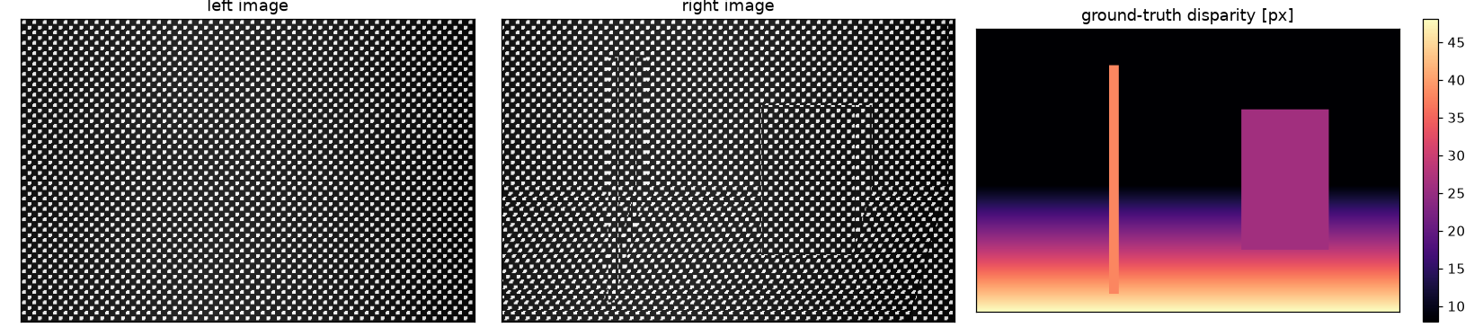
    d[(xx > 300) & (xx < 400) & (yy > 90) & (yy < 250)] = 26.0   # box
    d[(xx > 150) & (xx < 162) & (yy > 40) & (yy < 300)] = 38.0   # thin bar
    return d
Each feature breaks something. The slanted floor is sampled at different rates by the two views, so foreshortening violates one-to-one. The box edges generate occlusion. The thin bar violates the ordering constraint that scanline methods rely on.
The right image is a forward warp of the left by the true disparity, with a z-buffer, so occlusions appear on their own rather than being modelled:
for x, x2, d in zip(xs[ok], xr[ok], disp[y][ok]):
    if d > zbuf[y, x2]:          # nearer surface wins
        zbuf[y, x2] = d
        right[y, x2] = left[y, x]
Three textures
The same geometry is rendered three ways, because texture rather than geometry decides how hard the association is:
| texture | what it is | why |
|---|---|---|
| broadband | multi-scale noise | descriptors are individually discriminative; the easy case |
| dots | pseudo-random blobs | imitates an IR projector, as on a RealSense D435 |
| periodic | regular lattice | repetitive structure: brick, fencing, tiling. The hard case. |
2.2 Real pairs with ground truth
The synthetic right image is a warp of the left one, so every descriptor difference comes from resampling and added noise. Two real cameras differ in ways that cannot produce: different gain and vignetting, different noise, specular highlights that move with the viewpoint, surfaces that are not Lambertian.
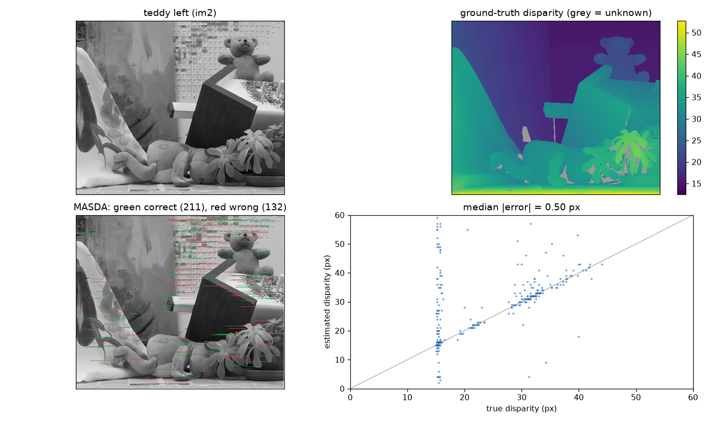
So the same matcher also runs on Teddy and Cones from the Middlebury 2003 stereo set. These are the pairs the stereo literature has been comparing on for twenty years, they are rectified, and they ship structured-light ground truth at quarter-pixel resolution with about 2-3% of pixels marked unknown. The dataset page states: “We grant permission to use and publish all images and disparity maps on this website.”
D. Scharstein and R. Szeliski (2003). High-accuracy stereo depth maps using structured light. CVPR, 195-202. doi:10.1109/CVPR.2003.1211354
Section 7 needs more than two scenes, so it also uses the six Middlebury 2005 scenes: Art, Books, Dolls, Laundry, Moebius and Reindeer, at third size. Those come from a different paper and carry their own citation:
D. Scharstein and C. Pal (2007). Learning conditional random fields for stereo. CVPR. doi:10.1109/CVPR.2007.383191
The 2005 two-view archives ship no documented disparity scale, so the factor of 3 is established rather than assumed: for a pixel at \(x\) in the left view with true disparity \(t\), the right view’s disparity map at \(x - t\) must also read \(t\). That identity holds to a median of 0.000 px at a scale of 3 and fails at every other integer, and it involves no matcher, so it cannot flatter the results.
Ground truth on real data needs one more piece of care than on synthetic data. Middlebury marks unknown disparity as zero rather than shipping a separate visibility mask, so a match landing on an unknown pixel has no correct answer to be compared against. Scoring those as wrong would charge the matcher for holes in the dataset, so they are counted separately and excluded from precision. On Teddy that is 10 matches out of 353.
3. Measuring the ambiguity
Descriptor degeneracy and matching ambiguity are different things, and only the second one matters.
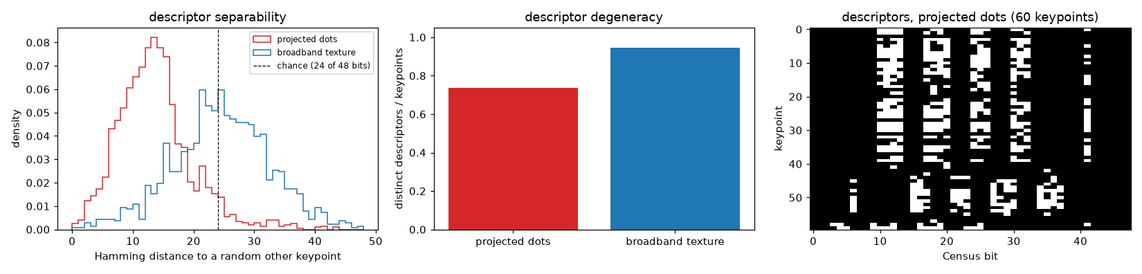
Over roughly 1400-2000 keypoints per image:
| texture | distinct descriptors | median score margin | margin < 0.05 |
|---|---|---|---|
| broadband | 95% | 0.750 | 4.7% |
| dots | 93% | 0.750 | 5.1% |
| periodic | 74% | 0.083 | 38.7% |
The score margin is best candidate minus runner-up, per left keypoint. It is what decides difficulty, and it is what a ratio test keys on. On the lattice the median margin is nine times smaller and 39% of keypoints have effectively tied candidates.
The distinct-descriptor count is misleading. The dot texture has 93% distinct descriptors, almost the same as broadband, yet this is supposed to be the ambiguous case. Anti-aliasing and sensor noise make every window unique as a bit pattern while leaving it uninformative as an identity. Counting distinct descriptors overstates how much information they carry; the margin measures it directly.
4. Implementation
The solver, in the notation above:
def masda(S, lam=-0.1, gam=-0.1, iters=30, damping=0.4, eps=1e-5):
    finite = np.isfinite(S)
    beta = np.where(finite, 0.0, -np.inf)
    rho  = beta.copy()

    for it in range(iters):
        # rho: a row's other options, or calling this measurement clutter
        comp = np.maximum(lam, top2_excluding(np.where(finite, beta, -np.inf), 1))
        new_rho = np.where(finite, (1 - damping) * (S - comp) + damping * rho, -np.inf)

        # beta: a column's other options, or calling this object misdetected
        comp = np.maximum(gam, top2_excluding(np.where(finite, new_rho, -np.inf), 0))
        new_beta = np.where(finite, (1 - damping) * (S - comp) + damping * beta, -np.inf)

        delta = max(np.nanmax(np.abs(new_rho - rho)),
                    np.nanmax(np.abs(new_beta - beta)))
        rho, beta = new_rho, new_beta
        if delta < eps:
            break

    belief = np.where(finite, beta + rho - S, -np.inf)
    return decide(S, belief, lam)
4.1 Reading out the answer
I got this wrong on the first attempt, and the mistake follows directly from the theory, so it is worth walking through.
I gated acceptance on \(b_{ij} > 0\). On problems with exactly tied candidates that returned zero matches, on problems whose optimum matched everything.
The belief measures an edge’s advantage over its competitors. When nothing has an advantage, every belief is \(\le 0\). That is also the condition under which the LP relaxation has no unique optimum, and uniqueness is exactly what Bayati, Shah and Sharma require for max-product to be correct on bipartite matching. So the degenerate case is not an edge case to patch around; it is where the guarantee stops.
Bayati, M., Shah, D., & Sharma, M. (2008). Max-Product for Maximum Weight Matching: Convergence, Correctness, and LP Duality. IEEE Transactions on Information Theory, 54(3), 1241-1251. doi:10.1109/TIT.2007.915695
Two questions were tangled together:
| question | answered by |
|---|---|
| which candidate? | the belief \(b_{ij}\), as an ordering. Its sign means nothing. |
| associate at all? | \(s(i,j)\) against \(\lambda\), which is what \(\lambda\) is for. |
So: order by belief, decide by \(\lambda\), require row and column to agree, then fill in greedily by belief over what is left.
def decide(S, belief, lam):
    order = np.argsort(-belief, axis=None)
    used_i, used_j, out = np.zeros(m, bool), np.zeros(n, bool), {}
    for flat in order:
        i, j = divmod(int(flat), n)
        if not np.isfinite(belief[i, j]):
            break
        if S[i, j] <= lam or used_i[i] or used_j[j]:
            continue
        out[i] = j
        used_i[i] = used_j[j] = True
    return out
The greedy fill is not cosmetic. Under near-ties every row’s best belief points at the same column, so requiring mutual agreement commits exactly one pair. Every greedily accepted edge has \(s > \lambda\) and two free endpoints, so it raises the objective. Adding it moved agreement with exhaustive search from 56/60 to 58/60 on problems small enough to enumerate.
5. Results against ground truth
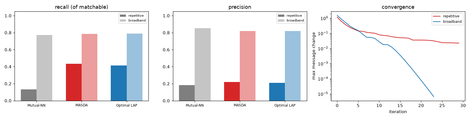
\(\lambda = \gamma = -0.1\), 30 iterations, damping 0.4. Recall is measured against attainable matches only: a left keypoint counts in the denominator only if its true correspondence is unoccluded and was itself detected in the right image. Counting the rest would charge the matcher for the detector’s misses.
5.1 Synthetic
broadband
| method | matches | correct | wrong | precision | recall | objective |
|---|---|---|---|---|---|---|
| Mutual-NN + ratio | 764 | 650 | 114 | 0.851 | 0.773 | 460.37 |
| MASDA | 807 | 661 | 146 | 0.819 | 0.786 | 476.67 |
| Optimal LAP (JV) | 807 | 662 | 145 | 0.820 | 0.787 | 476.67 |
dots
| method | matches | correct | wrong | precision | recall | objective |
|---|---|---|---|---|---|---|
| Mutual-NN + ratio | 854 | 690 | 164 | 0.808 | 0.801 | 491.28 |
| MASDA | 917 | 700 | 217 | 0.763 | 0.813 | 521.67 |
| Optimal LAP (JV) | 917 | 700 | 217 | 0.763 | 0.813 | 521.67 |
periodic
| method | matches | correct | wrong | precision | recall | objective |
|---|---|---|---|---|---|---|
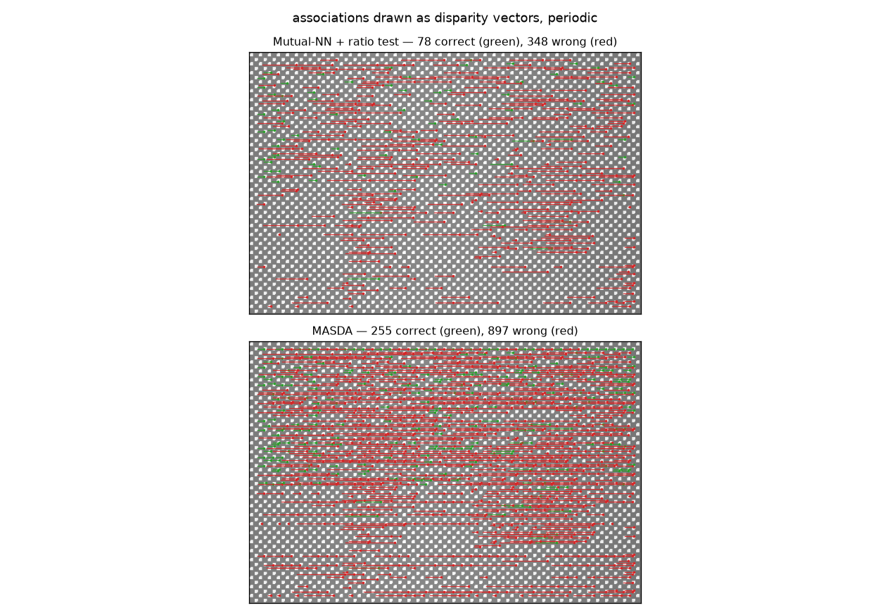
| Mutual-NN + ratio | 426 | 78 | 348 | 0.183 | 0.132 | 17.35 |
| MASDA | 1152 | 255 | 897 | 0.221 | 0.433 | 652.34 |
| Optimal LAP (JV) | 1151 | 243 | 908 | 0.211 | 0.413 | 656.68 |
5.2 Real pairs
Same matcher, same \(\lambda\) and \(\gamma\), same 30 iterations. “scorable” excludes matches landing on unknown ground truth. A match counts as correct within Middlebury’s standard 1 px threshold.
Teddy
| method | matches | scorable | correct | precision | recall | objective |
|---|---|---|---|---|---|---|
| Mutual-NN + ratio | 301 | 291 | 198 | 0.680 | 0.667 | 121.13 |
| MASDA | 353 | 343 | 211 | 0.615 | 0.710 | 153.62 |
| Optimal LAP (JV) | 353 | 343 | 209 | 0.609 | 0.704 | 153.62 |
Cones
| method | matches | scorable | correct | precision | recall | objective |
|---|---|---|---|---|---|---|
| Mutual-NN + ratio | 407 | 396 | 320 | 0.808 | 0.746 | 182.55 |
| MASDA | 441 | 430 | 336 | 0.781 | 0.783 | 204.98 |
| Optimal LAP (JV) | 441 | 430 | 334 | 0.777 | 0.779 | 204.98 |
The pattern from the synthetic scene survives: MASDA matches more than the ratio test (353 against 301, 441 against 407), gets more of them right (211 against 198, 336 against 320), and reaches the LAP objective exactly on both scenes. It again edges the exact solver on correct matches while tying on the objective, 211 against 209 and 336 against 334, which is tie-breaking rather than superiority.
Raw precision is much worse than on synthetic data, 0.615 and 0.781 against 0.849. Most of that gap is not the matcher’s fault, which took some digging to establish.
5.3 On real data the detector is the binding constraint
Keypoints are detected independently in the two images, and on real photographs Shi-Tomasi does not pick the same points twice. Only 48% of Teddy’s left keypoints have any right keypoint within 1 px of their true correspondence, and 51% on Cones. For the other half there is no correct answer available at any price, so a matcher that assigns them is wrong by construction.
Splitting MASDA’s errors accordingly:
| scene | correct | wrong, no correct answer existed | wrong, genuine matcher error |
|---|---|---|---|
| Teddy | 211 | 102 | 30 |
| Cones | 336 | 81 | 13 |
Precision restricted to keypoints that had an attainable answer is 0.876 on Teddy and 0.963 on Cones, against a raw 0.615 and 0.781. So of Teddy’s 132 wrong matches, 102 were forced by the detector and 30 were chosen badly.
This reorders the priorities in section 10. I had descriptor quality first, on the strength of the synthetic sweep. On real images, detector repeatability comes first: a matcher cannot recover a correspondence whose right-image endpoint was never proposed. It is also the cheaper fix, since it does not need a learned model, only a detector that agrees with itself across two views.
It is worth being clear that this is not a criticism of the numbers above. Raw precision is the number a downstream consumer actually experiences, so it is the number to report. The decomposition says where to spend effort next.
5.4 Ambiguity predicts precision on both kinds of data
The synthetic sweep’s central claim is that the score margin, best minus second best, predicts how well the matcher does. If that is a property of the problem rather than of my scene generator, real data should fall on the same curve.
It does. Teddy conveniently supplies a controlled comparison: its back wall is partly plain and partly covered in printed newspaper, at the same depth, in the same image, under the same lighting.
| region | median margin | precision | matches |
|---|---|---|---|
| synthetic periodic | 0.083 | 0.221 | 1152 |
| Teddy wall, printed | 0.417 | 0.514 | 138 |
| Teddy, whole scene | 0.542 | 0.615 | 343 |
| Teddy wall, plain | 0.667 | 0.804 | 46 |
| Cones, whole scene | 0.667 | 0.781 | 430 |
| synthetic broadband | 0.750 | 0.819 | 807 |
| synthetic dots | 0.750 | 0.763 | 917 |
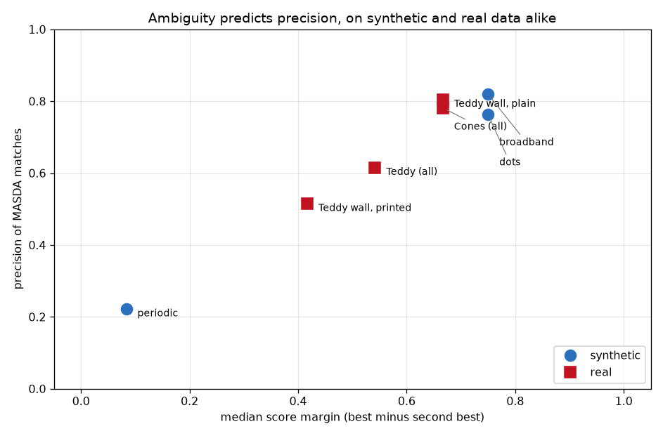
Precision rises with margin across both data sources, and the real points interleave with the synthetic ones rather than sitting apart from them. It is a trend and not a law: dots and broadband share a median margin of 0.750 but differ by 5 points of precision, and Teddy’s plain wall beats both from a lower margin. The median is a summary, so two scenes that agree on it can still differ in the tail.
The controlled part of the comparison is Teddy’s back wall. 59% of all Teddy’s wrong matches sit on it, the printed half and the plain half differ in nothing but texture, and precision differs by 29 points.
The synthetic lattice was not a strawman, then. It is the same failure that real repetitive texture produces, run at higher contrast so it can be measured cleanly. Real data does sit slightly below the synthetic trend at equal margin, which is what you would expect: two physical cameras add radiometric and specular differences that a warp cannot simulate, so a given margin buys a little less on real images.
5.5 Reading the numbers
MASDA reaches the optimum. Objective ratios against exact Jonker-Volgenant are 1.0000, 1.0000 and 0.9934. Loopy max-sum, with no guarantee available, lands on the LAP optimum on all three problems. That is not what “approximate inference on a loopy graph” leads you to expect.
On the lattice it also gets more correct matches than the exact solver, 255 against 243, while scoring slightly lower on the objective. The objective is a proxy, and maximising it exactly does not maximise correctness. The same thing happens on both real pairs, 211 against 209 and 336 against 334.
The gain over nearest-neighbour tracks ambiguity. Correct matches:
| texture | median margin | MASDA | Mutual-NN | ratio |
|---|---|---|---|---|
| broadband | 0.750 | 661 | 650 | 1.02× |
| dots | 0.750 | 700 | 690 | 1.01× |
| periodic | 0.083 | 255 | 78 | 3.27× |
| Teddy (real) | 0.542 | 211 | 198 | 1.07× |
| Cones (real) | 0.667 | 336 | 320 | 1.05× |
Where descriptors discriminate, uniqueness adds one or two percent and a ratio test is a perfectly reasonable matcher. Where they do not, MASDA finds 3.27× more correct correspondences. The real pairs sit in between at 5-7%, which fits: real texture is neither as clean as broadband noise nor as adversarial as a lattice.
Look at mutual-NN’s objective on the lattice: 17.35, against MASDA’s 652.34. The ratio test rejects so much that it barely scores at all. It is not trading badly; it is declining to trade.
Precision collapses for everyone. 0.221 for MASDA, 0.183 for mutual-NN, 0.211 for the exact optimum.
This is the result I find most useful. Uniqueness is real information and it is being used optimally here, since the exact solver does no better. But on genuinely repetitive texture the information is not in the descriptors, and constraint propagation cannot create it. What MASDA does is convert a refusal to answer into answers, most of which are wrong. Whether that helps depends on the consumer: a bundle adjustment with a robust loss will happily take 255 good matches out of 1152, while a naive triangulation will be poisoned.
So the claim is not that MASDA beats nearest-neighbour. It is that MASDA extracts everything the uniqueness constraint contains, which is a lot when descriptors are ambiguous and not enough when they are degenerate. That is what motivates adding further factors, which is section 7.
5.6 Damping
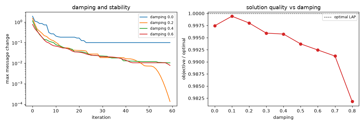
Undamped max-sum on the ambiguous problem does not settle; the largest message change plateaus instead of decaying. Damping of 0.3-0.5 stabilises it, and solution quality is flat across that range, staying within a fraction of a percent of optimal.
On real data (a D435 IR pair, 848×480, around 1100 keypoints) the messages never formally converge at any iteration budget, yet the decision is stable to four significant figures from 50 iterations and within 0.1% at 20. The oscillation is confined to messages that do not change the answer. Message convergence is not the property you actually need.
6. Speed: the representation decides it
The complexity argument is \(O(T \cdot E)\) against Jonker-Volgenant’s \(O(N^3)\). My first implementation did not benefit from it at all.
Written the obvious way, with messages in an \(m \times n\) array padded with \(-\infty\), MASDA is slower than scipy’s compiled Jonker-Volgenant:
| texture | nodes | edges | dense MASDA | JV (scipy) | ratio |
|---|---|---|---|---|---|
| broadband | 1377 | 3227 | 2633 ms | 1506 ms | 0.6× |
| dots | 1640 | 3947 | 5727 ms | 2521 ms | 0.4× |
| periodic | 2019 | 4556 | 9132 ms | 3962 ms | 0.4× |
With \(m \approx n \approx 1400\) the matrix holds about two million cells and 3227 real edges, so roughly 600× of the arithmetic goes into entries that are \(-\infty\). The \(O(T \cdot E)\) bound assumes an edge list. A dense array gives \(O(T \cdot m \cdot n)\) and vectorisation does not recover the difference.
6.1 Edge-list formulation
Put the messages on the edges. The only awkward part is that both updates need \(\max_{k \neq j}\) over a row or column, which is quadratic in row length if done directly. Three segment reductions answer it exactly in \(O(E)\):
def _seg_max_excluding(vals, idx, n):
    """Per-segment max with each element's own contribution removed, in O(E)."""
    m1 = np.full(n, -np.inf)
    np.maximum.at(m1, idx, vals)          # segment max
    at_max = vals >= m1[idx]              # m1 is the max, so >= means ==
    cnt = np.zeros(n, np.int64)
    np.add.at(cnt, idx[at_max], 1)        # how many attain it
    m2 = np.full(n, -np.inf)
    below = ~at_max
    if below.any():
        np.maximum.at(m2, idx[below], vals[below])   # max strictly below
    second = np.where(cnt > 1, m1, m2)
    return np.where(at_max, second[idx], m1[idx])
Three cases: an element below the max sees the max; an element at the max also sees the max, provided something else attains it; otherwise it sees the runner-up. Ties need handling rather than ignoring, since near-ties are the case of interest.
The solver is then five lines per iteration:
def masda_sparse(ei, ej, se, m, n, lam=-0.1, gam=-0.1, iters=30, damping=0.4):
    beta = np.zeros(len(se)); rho = np.zeros(len(se))
    for _ in range(iters):
        comp = np.maximum(lam, _seg_max_excluding(beta, ei, m))
        new_rho  = (1 - damping) * (se - comp) + damping * rho
        comp = np.maximum(gam, _seg_max_excluding(new_rho, ej, n))
        new_beta = (1 - damping) * (se - comp) + damping * beta
        rho, beta = new_rho, new_beta
    belief = beta + rho - se
    ...
Same messages, same damping, same belief, same decision rule. Only the representation differs.
6.2 What that gains
| texture | edges | dense | sparse | JV | vs dense | vs JV |
|---|---|---|---|---|---|---|
| broadband | 3227 | 2633 ms | 8.6 ms | 1506 ms | 308× | 176× |
| dots | 3947 | 5727 ms | 16.1 ms | 2521 ms | 357× | 157× |
| periodic | 4556 | 9132 ms | 17.2 ms | 3962 ms | 530× | 230× |
157-230× faster than compiled Jonker-Volgenant, from interpreted NumPy.
Quality is unchanged. Objectives match the dense solver to four decimals in all three cases, and correct-match counts differ by at most one out of several hundred, where the two orderings break ties differently: 661 against 661, 700 against 701, and 255 against 255. Both remain at the LAP optimum. The assignments are not bit-identical, and with tied beliefs they need not be.
On the real pairs the same ranking holds with a smaller margin:
| scene | nodes | edges | dense | sparse | JV | vs JV |
|---|---|---|---|---|---|---|
| Teddy | 1264 | 1683 | 495 ms | 5.5 ms | 156 ms | 28× |
| Cones | 1721 | 1591 | 1054 ms | 5.4 ms | 451 ms | 83× |
28-83× rather than 157-230×, because these problems are roughly half the size and Jonker-Volgenant is cubic while the sparse solver is linear in edges. The gap widens with problem size, which is the direction real systems move in.
As an independent check, the same algorithm as a C++ edge-list implementation on my own imagery (848×480 IR pair, about 1075 keypoints, 2882 candidate edges, 20 iterations) runs in 1.67 ms against a 33.3 ms frame budget at 30 Hz. The keypoint detector, at 21 ms, costs more than ten times as much.
6.3 The actual claim
MASDA’s cost is linear in the number of plausible associations, and in a geometrically constrained problem that is a small fraction of \(m \times n\). Here the epipolar band and disparity range cut roughly two million possible pairings down to 3200 candidates. Only a representation that exploits that sees any benefit.
This also reframes the comparison with an exact solver. It is not about accuracy, since Jonker-Volgenant is exactly as good and occasionally slightly better. It is that MASDA is anytime and incremental: it can be stopped early with a usable answer, its messages carry over between frames when the problem changes slightly, and it accepts factors that destroy the assignment structure, where a LAP solver cannot follow.
7. Can MASDA express the ordering constraint?
Scanline stereo methods use the ordering constraint: matches along a scanline should not cross. Plain MASDA cannot express it, which is a standing objection to using it for stereo. It can be added as a factor, the derivation is tidier than I expected, and whether it is worth using depends on which data you ask.
Two associations \((i,j)\) and \((i',j')\) cross iff \((x_i - x_{i'})(x_j - x_{j'}) < 0\). A matching is order-preserving exactly when no two of its pairs cross, so ordering decomposes into pairwise factors with no higher-order term. That is what makes it tractable.
Take \(\psi(c_e, c_f) = -\kappa\) when both edges are on and crossing, else 0. For a pairwise factor between binary variables only the difference of the outgoing message matters, and with \(\mu_f = m_f(1) - m_f(0)\):
\[\Delta_{\psi \to e} = \max(0, \mu_f - \kappa) - \max(0, \mu_f) = -\operatorname{clamp}(\mu_f,\, 0,\, \kappa)\]The ordering message is the conflicting edge’s own preference, clamped and negated. One scalar, constant time. I checked it against brute-force max-sum over 20000 random cases; agreement is 4×10⁻¹⁶.
Because these messages are additive on the edge they fold into the score. Writing \(o_e = -\sum_{f \in X(e)} \operatorname{clamp}(b_f, 0, \kappa)\) for the summed ordering pressure, the updates are the same two reductions with \(s + o\) substituted for \(s\). Nothing new has to be maintained. Crossing pairs depend only on geometry, so they are computed once; \(O(E_r^2)\) per scanline band here, and a Fenwick tree over the sorted \(j\) order would make it \(O(E_r \log E_r)\) if bands got dense.
\(\kappa\) stays finite. Thin foreground objects genuinely violate ordering, and a hard constraint would delete them. Damping goes up to 0.6, because these factors add loops that the bipartite convergence result does not cover.
7.1 On synthetic scenes it works and does not improve accuracy
The lattice is an unfair test on its own, because repetitive mistakes tend to be order-preserving: a region shifted by one period crosses nothing. So there is a second scene built for ordering, with nine thin bars at assorted depths over broadband texture, where errors do cross.
Both scenes are run over five random seeds, and what is reported is the paired difference against the same scene with the factor off. That is not decoration: the scene-to-scene spread below is ±31 correct matches against an effect of about 1, and single-scene runs of this experiment gave me opposite signs.
Thin bars, the scene built to favour ordering. Baseline: 512.0 ± 31.2 correct, 50.8 ± 11.3 crossings out of roughly 2800 same-band pairs.
| \(\kappa\) | Δ correct | Δ crossings |
|---|---|---|
| 0.1 | +1.6 ± 1.9 | −4.0 ± 3.0 |
| 0.4 | +1.0 ± 2.1 | −9.0 ± 6.1 |
| 0.8 | +1.0 ± 2.3 | −9.4 ± 6.0 |
Periodic. Baseline: 230.8 ± 18.8 correct, 227.2 ± 4.1 crossings out of ~9800.
| \(\kappa\) | Δ correct | Δ crossings |
|---|---|---|
| 0.1 | −7.2 ± 5.6 | −78.4 ± 14.9 |
| 0.4 | −6.0 ± 8.1 | −107.0 ± 18.1 |
| 0.8 | −7.4 ± 7.9 | −108.0 ± 17.1 |
The factor does what the derivation says it should. Crossings fall reliably and monotonically in \(\kappa\): by 18% on thin bars and 47% on the lattice.
Accuracy does not improve. On the scene built to favour ordering the change is one match in 512, smaller than its own spread across seeds, which reads as no effect. On repetitive texture it is consistently negative, −6 to −7 in every seed.
On this evidence I concluded the factor was not worth switching on. That conclusion was wrong, and section 7.2 is why.
7.2 On real data it does help, slightly
The synthetic answer is not the real answer, which I only found because two scenes with no error bars is not a measurement either. Middlebury 2005 supplies six more scenes with structured-light ground truth under the same licence, so the real side gets eight scenes and the same paired treatment.
Paired difference against the same scene with the factor off, over Teddy, Cones, Art, Books, Dolls, Laundry, Moebius and Reindeer:
| \(\kappa\) | Δ correct | Δ crossings | crossings retained |
|---|---|---|---|
| 0.1 | +1.9 ± 2.3 | −12.4 ± 11.7 | 0.75× |
| 0.3 | +2.1 ± 2.3 | −16.8 ± 16.6 | 0.64× |
| 0.8 | +2.2 ± 2.5 | −17.6 ± 16.5 | 0.62× |
At \(\kappa = 0.3\) the factor is better on 6 scenes, worse on 1, unchanged on 1. The mean is +2.1 correct per scene against baselines of 114 to 336, so about +0.9%, with a standard error of 0.85 and a one-sample \(t\) of 2.49, \(p = 0.042\).
That is a small effect with marginal significance on eight scenes, and I would not build anything on the \(p\)-value alone. What makes it believable is the consistency: it never costs more than one match, and it cuts crossings by a third on every scene.
So the answer is the opposite of what the synthetic scenes said. On real imagery an ordering factor is worth switching on. It is cheap, it removes a third of the crossings, and it returns about one percent more correct matches.
7.3 Why the two disagree
Matches \((i,j)\) and \((i',j')\) with \(x_i < x_{i'}\) cross iff \(x_j > x_{j'}\), that is
\[d_{i'} - d_i \;>\; x_{i'} - x_i\]A crossing needs the disparity difference to exceed the horizontal separation. With disparities confined to a range of width \(d_{\max} - d_{\min}\), crossings are only possible between keypoints closer together in \(x\) than that width. That bound is real, and it was my original explanation for why ordering was redundant: the disparity gate has already forbidden most crossings, so there is little left to fix.
The eight real scenes do not support that explanation. If gate width governed the crossing rate, the six scenes gated at 80 px should cross more than the two gated at
- The correlation is +0.50 with \(p = 0.21\), which on eight points is nothing.
What does predict the crossing rate is the error rate:
| scene | precision | crossings / same-band pair |
|---|---|---|
| Cones | 0.781 | 1.3% |
| Dolls | 0.689 | 2.5% |
| Books | 0.704 | 4.6% |
| Teddy | 0.615 | 4.6% |
| Moebius | 0.680 | 4.9% |
| Art | 0.489 | 5.1% |
| Reindeer | 0.592 | 7.4% |
| Laundry | 0.301 | 9.3% |
Spearman \(\rho = -0.86\), \(p = 0.0065\). Crossings are mostly a symptom of wrong matches, not an independent property of the geometry. That is why penalising them removes wrong matches, and why the effect is larger on the scenes that need it most.
It also explains the synthetic result, and why it pointed the wrong way. On a periodic lattice the errors are order-preserving: a patch matched one period to the left crosses nothing, because every keypoint in it shifts by the same amount. So the factor finds no wrong matches to remove and spends its influence perturbing correct ones, which is exactly the −6 it costs. The lattice is not a hard case for ordering, it is a case where ordering is blind.
I had flagged the lattice as an unfair test and then built the thin-bars scene to compensate. That was the right instinct and it was not enough: thin bars violate ordering legitimately, so they penalise the factor from the other direction. Between a scene where ordering cannot see the errors and a scene where the true answer breaks the constraint, both of my synthetic tests were adversarial to it in ways real scenes are not.
Ordering is therefore expressible, cleanly, inside the existing closed form, cheap enough to leave on, and worth about a percent on real imagery. I would still expect it to matter more where the gating is weak: an uncalibrated pair, or two-dimensional temporal association, where nothing constrains ordering for free.
8. Comparison with existing work
Jonker-Volgenant / Hungarian. Exact, \(O(N^3)\), and here at least as good as MASDA everywhere. For a pure assignment problem of moderate size, use it. MASDA earns its place when you intend to add factors that stop the problem being a LAP.
Jonker, R., & Volgenant, A. (1987). A shortest augmenting path algorithm for dense and sparse linear assignment problems. Computing, 38(4), 325-340. doi:10.1007/BF02278710
SPADA / sum-product data association. Produces marginal association probabilities rather than a MAP assignment, at higher cost. If the consumer wants soft weights, for a PDA-style tracker or a differentiable pipeline, that is the right choice. Stereo wants a decision per keypoint, so MAP is what is needed.
Sinkhorn and optimal transport, as in SuperGlue. Structurally very close: soft one-to-one assignment with dustbins, which are \(\lambda\) and \(\gamma\) under another name. Sinkhorn is the entropy-regularised relaxation and max-sum is its zero-temperature limit. SuperGlue’s real advantage is that its scores come from a learned attention network instead of a hand-designed \(s(i,j)\), and its dustbin costs are learned rather than set. That points straight at the weakest part of what I have here.
Sarlin, P.-E., DeTone, D., Malisiewicz, T., & Rabinovich, A. (2020). SuperGlue: Learning Feature Matching with Graph Neural Networks. CVPR. arXiv:1911.11763
Semi-global matching and dense stereo. A different problem, and worth saying why sparse matching is not simply the worse option. Dense stereo assigns a disparity to every pixel with a smoothness prior on the pixel grid; per scanline, one-to-one with occlusion is solved exactly by dynamic programming in \(O(W \cdot D)\), and DP also encodes the ordering constraint that MASDA needs a factor for. If you want a dense disparity map, MASDA is the wrong tool. Sparse matching is the right tool when you want a few hundred well-localised sub-pixel correspondences to feed geometry, such as odometry, calibration or structure, rather than a depth image.
Hirschmüller, H. (2008). Stereo Processing by Semiglobal Matching and Mutual Information. IEEE TPAMI, 30(2), 328-341. doi:10.1109/TPAMI.2007.1166
ELAS is worth mentioning too: it uses a triangulated set of robustly matched support points as a prior for dense estimation, which is close to the sparse-then-densify arrangement a MASDA front end would naturally feed.
Geiger, A., Roser, M., & Urtasun, R. (2011). Efficient Large-Scale Stereo Matching. ACCV 2010, LNCS 6492, 25-38. doi:10.1007/978-3-642-19315-6_3
9. Advantages
Where MASDA is the right choice:
- Cost is linear in plausible associations rather than in \(m \times n\). With geometric constraints cutting candidates to about 2.3 per keypoint, the sparse form runs 157-230× faster than an exact LAP solver at the same quality.
- It is optimal, or indistinguishable from optimal, on these problems without needing to be.
- It is anytime. A handful of iterations gives a usable answer, and the decision stabilises well before the messages do.
- It extends, and this is the main reason to prefer it over an exact LAP solver. Adding an ordering, smoothness or temporal factor keeps a factor graph a factor graph, whereas it stops being an assignment problem. section 7 is the demonstration: a new pairwise constraint cost one clamped scalar per conflicting edge, no change to the update structure, and it pays for itself on real pairs.
- Clutter and misdetection are first-class rather than post-hoc thresholds, which matters when occlusion makes 30% of keypoints unmatchable.
Where it is not:
- The correctness guarantee is conditional and the condition is not always met. Bayati, Shah and Sharma require the LP relaxation to have a unique optimum; exactly tied scores break that, and repetitive texture is where ties come from. In practice it still reached the optimum on both real pairs and came within 0.7% of it on the lattice, but nothing in the theory promised that.
- It cannot create information. On degenerate texture it produces confident wrong answers where a ratio test produces none, and which of those is preferable is a property of the consumer.
- \(\lambda\) and \(\gamma\) are hand-set. The scale here is interpretable, which helps, but that is not the same as calibrated.
10. What would improve the matcher
Ranked by how much I expect them to matter. Real data reordered this list; the first item was not on it at all before section 5.3.
Detector repeatability. Only about half of the left keypoints on Teddy and Cones have a right-image keypoint within a pixel of their true correspondence, and the matcher cannot recover a correspondence that was never proposed to it. That single number bounds recall below 51% before matching starts, and it accounts for 102 of Teddy’s 132 errors. Concretely: detect in one image and track into the other rather than detecting twice, or lower the detector threshold to over-propose on the right and let \(\gamma\) discard the surplus, which is what the misdetection term is for. This needs no learned model and no new mathematics, which is why it goes first.
Better scores. \(s(i,j)\), \(\lambda\) and \(\gamma\) are the weakest part of this by a wide margin. Everything in section 5 says the constraint machinery is already extracting what it can, and the shortfall is in the evidence being fed to it. A small model over descriptor distance, vertical residual, response ratio and local texture energy, trained against ground truth to output a calibrated log-likelihood ratio, would change the numbers more than any refinement of the message passing. SuperGlue’s results point the same way.
Disparity smoothness over a neighbourhood graph. Neighbouring keypoints on the same surface should have similar disparity, and nothing here uses that. It is the largest piece of information currently ignored. Before deriving new messages the cheap version is worth trying: match, fit a robust disparity surface over a Delaunay triangulation of the left keypoints, rescore, rematch. I have tried a nearest-neighbour-graph version of this and it did not help, but the prior was fitted from the same matches it then judged, which makes it close to self-confirming. A properly triangulated version with a robust cost is a different experiment.
Sub-pixel disparity. Depth accuracy depends on this more than on anything else. Keypoint positions are refined sub-pixel, but disparity is currently just the difference of two independently refined positions rather than a fit to the correlation surface between them.
Unrolled training. Whether \(T\) max-sum iterations can be unrolled with a soft-max relaxation and trained end to end. Structurally that is what SuperGlue does with Sinkhorn in the zero-entropy limit, so the interesting question is whether the max-sum version is competitive with fewer parameters.
Temporal association. The same machinery for frame-to-frame matching, for ego-motion. The search is two-dimensional there, so nothing constrains ordering for free and \(k\) is genuinely large, which gives a motion prior from IMU-derived rotation compensation something to prune.
A caveat on all of the above. Three synthetic textures and eight real scenes is not a benchmark, and images around 450×375 are small by current standards. What I would expect to hold generally is the shape of the results: the gain over a ratio test tracks ambiguity, loopy max-sum lands on the LAP optimum, precision collapses under degeneracy for every method including the exact one, and on real images the detector binds before the matcher does. The specific figures are what this code did on these scenes.
The ordering result is the one I would trust least and the one I would most want someone to repeat. It is about a 1% effect, significant at \(p = 0.042\) on eight scenes, and it points the opposite way from what my synthetic scenes said. That is enough to switch the factor on, since it is nearly free, and not enough to call it settled.