Faster Data Association with Max-Sum Loopy Belief Propagation (MASDA)

This presents a data association algorithm I call MASDA (Max-Sum Algorithm Data Association) which relies on message passing in a factor graph.

I derived the formula presented here using the very same approach as in the paper:

Givoni, Inmar & Frey, Brendan. (2009). A Binary Variable Model for Affinity Propagation. Neural Computation. 21. 1589-1600. 10.1162/neco.2009.05-08-785.

Further, I describe the relation to SPADA (Sum-Product Algorithm Data Association). The Paper Message Passing Algorithms for Scalable Multitarget Tracking by Florian Meyer discusses SPADA for object tracking purposes in detail.

Meyer, Florian & Kropfreiter, Thomas & Williams, Jason & Lau, Roslyn & Hlawatsch, Franz & Braca, Paolo & Win, Moe. (2018). Message Passing Algorithms for Scalable Multitarget Tracking. Proceedings of the IEEE. 106. 221-259. 10.1109/JPROC.2018.2789427.

At last I provide a naive implementation in python to link the math to a working example for better comprehension.

Introduction

Data association is a fundamental problem in many fields, particularly in robotics, computer vision, and autonomous systems. It involves the challenging task of correctly linking incoming data (e.g., sensor measurements) to existing entities or tracks.

Example 1: Measurement-to-Object Association

Consider a scenario in autonomous driving or surveillance where a vehicle is equipped with sensors (e.g., radar, lidar, camera) that detect objects in its environment. At each time step, these sensors generate a set of ‘measurements’ – detections of potential objects. Simultaneously, the system maintains a set of ‘objects’ (or tracks) that it believes exist and is currently monitoring. The core challenge of measurement-to-object association is to determine which new measurement corresponds to which existing object, or if a measurement represents a new, previously unobserved object (a ‘birth’), or if an existing object was not detected in the current scan (a ‘missed detection’ or ‘misdetection’), or if a measurement is spurious (e.g., ‘clutter’).

For example, suppose a radar detects a blob at a certain position. In that case, the data association algorithm must decide if this blob is the same car it measured in a previous scan, a newly appeared pedestrian, or just sensor noise. Incorrectly associating a new measurement with an old track can lead to track swapping, where the system believes it’s still tracking the original object but is actually tracking a different one. This can have severe consequences, such as an autonomous vehicle mispredicting the behavior of surrounding traffic.

Example 2: Data Association in Simultaneous Localization and Mapping (SLAM)

In SLAM, a mobile robot or agent builds a map of an unknown environment while simultaneously estimating its own position within that map. Data association in SLAM is crucial for both map consistency and accurate localization. When a robot observes a feature (e.g., a corner, a door, a landmark) with its sensors, it needs to determine whether it corresponds to a feature already present in its growing map or is a new feature to be added. This is known as feature association or loop closure detection (when the robot revisits a previously mapped area).

If the robot incorrectly associates a newly observed feature with an existing map feature that is actually different, it can introduce significant errors into the map (e.g., duplicate features, skewed map geometry) and its own estimated pose. Conversely, if it fails to associate a revisited feature, it might incorrectly believe it’s in a new area, leading to an ever-growing, inconsistent map. Correct data association is paramount for closing loops in the map and maintaining a globally consistent representation of the environment.

Data association algorithms are also needed in other fields, such as medicine, statistics, biology, and weather forecasting, to name a few. As the terminology differs in those fields, I will stick to the terms measurements and detections for the entities that describe the state of the system perceived without prior knowledge from a previous scan. These might be raw measurements, such as positions, or already processed data, such as clusters and features. Objects describe an accumulated, maybe “learned” state or just a previous state of the system. In a multi-sensor setup, with overlapping fields of view, where multiple scans shall be matched to each other, the term “measurements” might describe the data coming from one sensor, and the term “objects” describes the data received from another.

Objects and measurements are considered throughout this article as independent and identically distributed (i.i.d.).

Hungarian-Derived Algorithms

Hungarian-derived algorithms (e.g., the Munkres algorithm for the Assignment Problem) are classic methods for solving optimal assignment problems, which can be framed as a data association task where the goal is to find a one-to-one mapping between two sets of items to minimize total cost or maximize total similarity. While powerful, their computational complexity grows in many applications too large.

The standard Hungarian algorithm has a polynomial time complexity, typically O(N^3) for N items. In scenarios with a large number of measurements and objects, or when running in real-time on resource-constrained systems, this can be computationally prohibitive. Real-world applications often involve hundreds or thousands of potential associations.

The Jonker-Volgenant Algorithm

The Jonker-Volgenant Algorithm was developed to improve upon the Hungarian Algorithm and is now the preferred method for solving the Linear Assignment Problem (LAP) for large, square cost matrices. Complexity: Although both algorithms can achieve a theoretical worst-case time complexity of \(O(n^3)\) (where \(n\) is the number of rows/columns of the cost matrix) in their improved versions, the Jonker-Volgenant method was fundamentally designed to be practically more efficient.

Factor Graphs for Data Association

Using a factor graph to solve the association problem offers several significant advantages, particularly for complex scenarios like data association in robotics or computer vision:

Factor graphs provide a highly intuitive and graphical way to represent complex probabilistic models. You can visually see the variables (e.g., whether a measurement is associated with an object, or is clutter) and the factors (e.g., the similarity score between them, or the constraints that govern assignments). This clarity helps in designing and understanding the problem’s structure.

The factor graph structure is highly modular. Each factor represents a local function or constraint, allowing for easy inclusion or modification of different aspects of the problem without redesigning the entire system. For instance, adding a new type of constraint (e.g., objects cannot be too close to each other) or a different similarity metric simply means adding a new factor or modifying an existing one.

The factor graph below and the notation is used throughout this article.

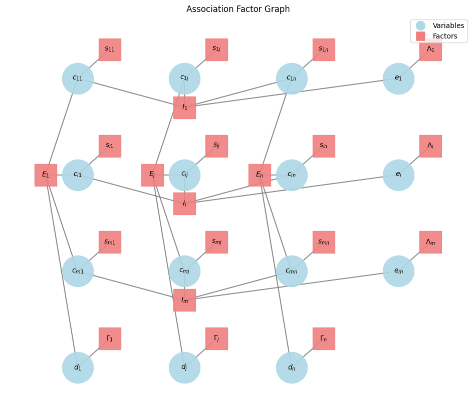
Factor graphs explicitly show the dependencies between variables. In data association, this means clearly delineating how individual association decisions (\(c_{ij}\)), clutter decisions (\(e_i\)), and misdetection decisions (\(d_j\)) are influenced by similarity scores and, crucially, by mutual exclusivity constraints (\(I_i\) and \(E_j\)). This explicit representation is vital for ensuring that the algorithm respects all rules of the problem.

Factor graphs are the natural framework for message-passing algorithms like Max-Sum (used in MASDA) or Sum-Product (used in SPADA). These iterative algorithms allow local information (messages) to propagate throughout the graph, enabling the system to infer global states (the best assignment) by combining local preferences and constraints. This is often more scalable and robust than traditional methods that might struggle with the combinatorial explosion of possibilities.

Data association is inherently a combinatorial problem. Factor graphs, along with message-passing algorithms, offer an efficient (though often approximate for loopy graphs) way to search this vast space for optimal or near-optimal solutions, by avoiding the need to enumerate all possible assignments.

Factor graphs can seamlessly integrate various types of information, including:

• Unary potentials: Costs/similarities for individual assignments (\(S_{ij}\)), clutter (\(\Lambda_i\)), or misdetections (\(\Gamma_j\)).
• High-order potentials/constraints: Complex relationships involving multiple variables, such as the mutual exclusivity constraints (\(I_i\) and \(E_j\)) that ensure each measurement associates with at most one object/clutter, and each object associates with at most one measurement/misdetection.

Depending on the message-passing algorithm used:

• Max-Sum (MASDA) can find the Maximum A Posteriori (MAP) assignment, giving you the single most likely set of associations.
• Sum-Product (SPADA) can compute marginal probabilities for each possible association, providing a rich, probabilistic understanding of the uncertainty in the assignments, which is crucial for robust decision-making in real-world systems.

Factor graphs provide a powerful, flexible, and mathematically rigorous framework for modeling data association problems, allowing for the application of efficient inference algorithms that can handle complex constraints and deliver either a single optimal assignment or a full probabilistic understanding of potential associations.

SPADA (Sum Product Algorithm Data Association) and MASDA (Max-Sum Algorithm Data Association)

SPADA is a method for solving data association problems using the Sum-Product Algorithm (SPA), also known as Belief Propagation. While the Max-Sum algorithm (which this page is demonstrating below) aims to find the single best assignment (the maximum a posteriori or MAP estimate), the Sum-Product Algorithm aims to compute marginal probabilities for each possible assignment. This means SPADA provides a more complete probabilistic understanding of the associations at the cost of higher computational efforts.

Here’s a breakdown:

Instead of just finding the most likely configuration, SPADA computes the marginal probability for each potential association variable (e.g., the probability that measurement i is associated with object j). It operates on a factor graph, similar to Max-Sum, but the messages passed between nodes represent probability distributions (or likelihoods in the log-domain), rather than just ‘scores’ or ‘costs’.

Factor Graph Representation

Variable nodes represent potential associations (e.g., \(c_{ij}\) for associating measurement \(i\) with object \(j\), \(e_i\) for clutter, \(d_j\) for misdetection). Factor nodes represent the relationships and constraints between these variables (e.g., similarity costs, mutual exclusivity constraints).

Messages in SPADA

In the Sum-Product Algorithm, messages are typically represented as functions (or vectors) over the possible states of the variable they are being sent to.

Variable-to-Factor Messages: A message from a variable node to a factor node is the product of all incoming messages from other factor nodes connected to that variable.

Factor-to-Variable Messages: A message from a factor node to a variable node is computed by taking the product of the factor’s function with all incoming messages from other variable nodes connected to that factor, and then summing (or integrating) over all variables except the recipient variable. The ‘sum’ in Sum-Product refers to this marginalization step, contrasting with the ‘max’ in Max-Sum where maximization is performed.

Messages are iteratively passed until they converge (or for a fixed number of iterations). Once messages converge, the belief (or marginal probability distribution) for each variable node can be computed by multiplying all messages received by that variable node. These beliefs represent the marginal probabilities of each possible association (e.g., \(P(c_{ij}=1)\), \(P(e_i=1)\), \(P(d_j=1)\)).

Key Differences from Max-Sum (MASDA)

Max-Sum aims for MAP (most likely assignment), SPADA aims for marginal probabilities. Therefor Max-Sum uses max and sum operations while SPADA uses sum and product operations (or log-sum-exp and sum in the log-domain to prevent underflow and allow for the benefits of addition instead of multiplication). Max-Sum typically gives a hard assignment (0 or 1 for each \(c_{ij}\)). SPADA provides probabilities (values between 0 and 1) for each association. SPADA’s probabilistic output can be more robust in ambiguous situations, as it quantifies the uncertainty of each association.

Advantages of SPADA

SPADA provides a richer understanding of the association uncertainty, which can be crucial for downstream decision-making in autonomous systems. When multiple assignments are plausible, SPADA can assign non-zero probabilities to each, reflecting the ambiguity. The marginal probabilities can be used to calculate expected values, variances, or for more sophisticated decision-making processes.

Applications

SPADA is used in various data association contexts, particularly where a nuanced, probabilistic understanding of associations is required. This includes multi-target tracking, sensor fusion, and certain aspects of SLAM where evaluating the likelihood of different map updates is important. In essence, while the Max-Sum algorithm helps you find the best way to associate measurements to objects, SPADA helps you understand how likely each possible association is, offering a more complete picture of the uncertainty in the system.

MASDA

MASDA, or Max-Sum Algorithm Data Association, is an iterative message-passing algorithm used to find the most likely (Maximum A Posteriori or MAP) assignment in data association problems. It operates on a factor graph, which visually represents the variables involved and the relationships (factors) between them.

Factor Graph Structure

The factor graph structure for MASDA remains the same as before. The architecture and the derivation below follows closely the ideas in A Binary Variable Model for Affinity Propagation

Variable Nodes (Circles, e.g., \(c_{ij}\), \(e_i\), \(d_j\)): These represent the decisions or unknowns we want to infer:

• \(c_{ij}\): Binary variables indicating whether measurement \(i\) is associated with object \(j\) (\(c_{ij}=1\)) or not (\(c_{ij}=0\)).
• \(e_i\): Binary variables indicating whether measurement \(i\) is ‘clutter’ (not associated with any existing object).
• \(d_j\): Binary variables indicating whether object \(j\) is ‘misdetected’ (not associated with any measurement).

Factor Nodes (Squares, e.g., \(s_{ij}\), \(\Lambda_i\), \(\Gamma_j\), \(E_j\), \(I_i\)): These represent functions that define relationships, costs, or constraints between the connected variable nodes:

Similarity Factors (\(s_{ij}\)): These factors (e.g., \(S_{ij}(c_{ij})\)) encode the cost or similarity of associating measurement \(i\) with object \(j\). When \(c_{ij}=1\), its value is \(s(i,j)\) (the similarity score); otherwise, it’s 0. These are essentially priors for specific associations.

Clutter Factors (\(\Lambda_i\)): These factors (e.g., \(\Lambda_i(e_i)\)) represent the cost or prior probability that measurement \(i\) is clutter. If \(e_i=1\), its value is \(\lambda(i)\); otherwise, it’s 0.

Misdetection Factors (\(\Gamma_j\)): These factors (e.g., \(\Gamma_j(d_j)\)) represent the cost or prior probability that object \(j\) is misdetected. If \(d_j=1\), its value is \(\gamma(j)\); otherwise, it’s 0.

Constraint Factors (\(I_i\) and \(E_j\)): These are crucial for enforcing the rules of data association:

Measurement Constraint Factors (\(I_i\)): (For each measurement \(i\)) This factor ensures that each measurement \(i\) is either associated with exactly one object, or it is declared as clutter (\(e_i=1\)). The function \(I_i(c_{i1}, \dots, c_{iN}, e_i)\) evaluates to \(-\infty\) (a very high cost in the log-domain, making it impossible) if \(e_i + \sum_j c_{ij} \neq 1\). Otherwise, it’s 0.

Object Constraint Factors (\(E_j\)): (For each object \(j\)) This factor ensures that each object \(j\) is either associated with exactly one measurement, or it is declared as misdetected (\(d_j=1\)). The function \(E_j(c_{1j}, \dots, c_{Nj}, d_j)\) evaluates to \(-\infty\) if \(d_j + \sum_i c_{ij} \neq 1\). Otherwise, it’s 0.

Objective Function:

The goal of MASDA is to find the assignment of all \(c_{ij}\), \(e_i\), and \(d_j\) variables that maximizes the total score (or minimizes total cost) as defined by the objective function \(\mathcal{S}\):

This function sums up all the similarity/cost factors for associations, clutter, misdetections, and critically, applies the penalties for violating the mutual exclusivity constraints.

Message Passing (The “Max-Sum” part):

MASDA works by iteratively passing “messages” between the variable and factor nodes. These messages represent beliefs or preferences about the state of the variables. The algorithm is typically run in the log-domain, so “sum” replaces “product” and “max” replaces “sum” from the original Sum-Product algorithm. The messages passed are essentially scores.

Variable-to-Factor Messages: A variable node \(x\) sends a message to a factor node \(f\) that is the sum of all incoming messages to \(x\) from other factor nodes (excluding \(f\)).

Factor-to-Variable Messages: A factor node \(f\) sends a message to a variable node \(x\) by taking the maximum over all possible assignments of its other connected variables, adding its own function value, and summing all messages from other variables (excluding \(x\)).

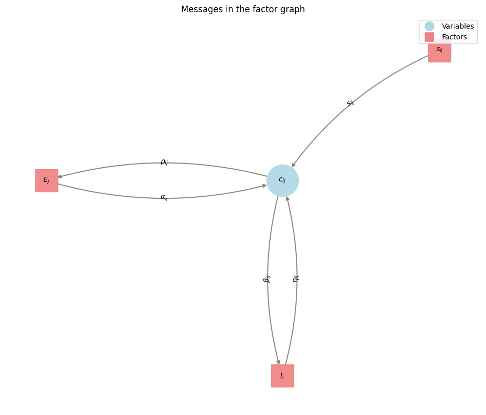
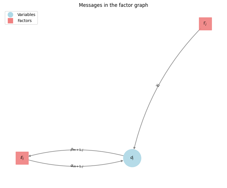
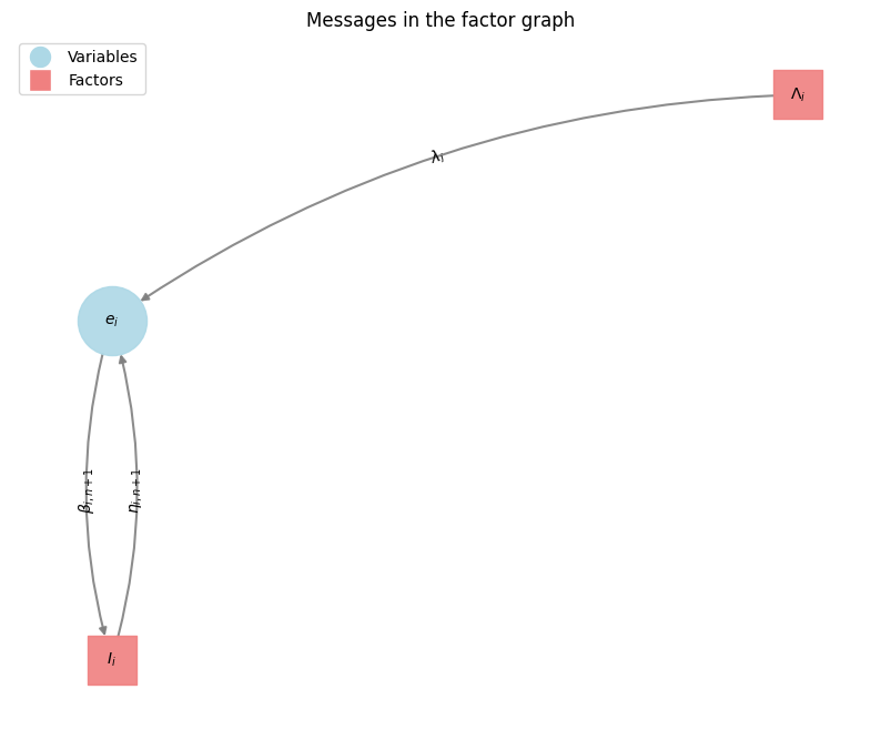
The messages for the binary nodes \(c_{ij}\), \(e_i\), \(d_j\) can be theoretically expressed with with a two-valued vector. But this is for our purpose of finding the best association, a MAP estimate, not necessary. Propagating its differences, a scalar, is enough as the two values can be recovered from this difference up to an additive constant factor.

For example: The message from Factor \(I_j\) to the variable \(c_{ij}\) is denoted with \(\beta_{ij}(m)\) \(\beta_{ij}(m) = \mu_{c_{ij} \rightarrow I_i}(m)\) where \(m \in \{0,1\}\) The scalar message difference is denoted \(\beta_{ij} = \beta_{ij}(1) - \beta_{ij}(0)\) This notation is also used for the messages \(\alpha_{ij}\), \(\rho_{ij}\) and \(\eta_{ij}\)

Variable to Factor Messages

These messages are just computed by the sum of the incoming messages, as stated above.

In order to simplify the notation we substitude the variables of the nodes and factors as follows

Message To \(I\)

for \(c_{ij} = 1\):

for \(c_{ij} = 0\):

Scalar message

Message To \(E\)

The derivation is similar to \(I\)

There is no message to the \(S\) factor at it is used as a prior.

Factor to Variable Messages

We make use of the previously given factor to variable message update equation. Again, we will fix \(c_{ij}\) to \(0\) and \(1\) respectively. Any combination that violates the constraints evaluates to \(\infty\) and is non optimal.

From \(I\)

This constrains only rows, ensuring that one measurement is associated to one object or is clutter/birth.

for \(c_{ij} = 1\), the association case

This is as only one node in the neighborhood of \(I\) can be set to \(1\)

for \(c_{ij} = 0\), the non association case

Exactly one of the variables in a row must be set to \(1\), all the others must be set to \(0\)

The scalar message is

From \(E\)

This can be derived similarly as the constraint is the same but ensures that only one vertical node is active (ensuring that one object is associated to one measurement)

for \(c_{ij} = 1\) the association case

for \(c_{ij} = 0\), the non association case

Exactly one of the variables in a column must be set to \(1\), all the others must be set to \(0\)

The scalar message is

From \(S\)

The scalar message send from the \(S_{ij}\) function is always the similarity between \(i\) and \(j\), since \(s(i,j) = S_{ij}(1) - S_{ij}(0)\)

Summary

As

Combined

The belief

Is just the sum of the messages towards a variable node.

Belief association between measurement and object

Belief measurement is clutter or a new born object

Belief that an object was misdetected

Iterative Process

These messages \(\beta\) and \(\rho\) are iteratively updated until convergence or for a fixed number of iterations. As messages propagate, information about similarities, clutter/misdetection likelihoods, and constraints are shared across the graph. This allows the algorithm to find a globally consistent assignment that satisfies as many preferences and constraints as possible.

Final Beliefs and Assignment

After message passing, the final “belief” for each variable (e.g., \(c_{ij}\)) is computed by summing all incoming messages to that variable from its connected factors. The assignment that maximizes this belief for each variable is chosen, resulting in a set of binary associations, cluttered measurements, and misdetected objects.

In essence, MASDA provides an approximate solution to the data association problem by intelligently propagating local preferences and global constraints throughout the system, ultimately finding the most probable assignment given all available information.

Computational Complexity: MASDA vs. Jonker-Volgenant

The Jonker-Volgenant algorithm is a highly optimized method for solving the Linear Assignment Problem. Its computational complexity is typically O(N^3), where N is the number of items to be assigned (e.g., number of measurements or objects, after potentially augmenting the problem to handle clutter and misdetections).

This complexity holds when you have a well-defined cost matrix and are seeking a strict one-to-one assignment that minimizes total cost. JV is known for its speed and guaranteed optimality for LAP.

MASDA is an iterative inference algorithm, a form of Belief Propagation. Its complexity, similar to SPADA, depends on the graph structure and the number of iterations.

In a data association factor graph with \(M\) measurements and \(N\) objects, computing messages for MASDA involves performing ‘max’ operations over the neighbors of each node. The complexity per iteration is roughly proportional to the number of edges and the number of states a variable can take within a factor, often scaling similarly to O(M * N * K), where K is related to the maximum degree of nodes or the size of variable domains within factors.

When applied to loopy factor graphs (which are common in data association), is an approximate inference algorithm. It’s not guaranteed to converge to the globally optimal MAP assignment, nor is it guaranteed to converge at all in all cases. In practice, it’s typically run for a fixed number of iterations (e.g., T iterations). Thus, the total practical complexity becomes O(T * M * N * K).

Note that for our purpose of data association, K is set 1.

Key Differences:

JV provides a provably optimal solution for the Linear Assignment Problem. MASDA provides an approximate solution to the MAP problem on loopy graphs. While often very good in practice, its optimality is not guaranteed.

MASDA’s iterative, message-passing nature allows it to more naturally incorporate complex constraints (like the one-measurement-per-object and one-object-per-measurement constraints, along with clutter and misdetection) directly into the factor graph structure, without needing extensive matrix augmentation as JV often does.

For pure LAP, JV’s O(N^3) is very efficient for moderate N. However, for very large N (where N is the number of potential associations), if the factor graph for MASDA is sparse and only a small number of iterations T are needed, MASDA can offer better practical scaling for certain types of problems that JV would struggle to model directly without significant pre-processing or approximation.

In essence, if your data association problem can be accurately and effectively framed as a pure Linear Assignment Problem, the Jonker-Volgenant algorithm will provide a guaranteed optimal solution. However, if the problem involves more complex probabilistic dependencies, non-strict one-to-one assignments, or requires intrinsic handling of clutter and misdetections without heavy augmentation, MASDA provides a flexible framework that can yield good approximate solutions, often with even faster runtime for a fixed number of iterations.

Computational Complexity: MASDA vs. SPADA

Both SPADA (Sum-Product Algorithm Data Association) and MASDA (Max-Sum Algorithm Data Association) are iterative message-passing algorithms operating on factor graphs.

SPADA generally involves higher computational efforts compared to MASDA because it aims to compute marginal probabilities for each possible assignment, rather than just the single most likely assignment. While not explicitly stated with a formula in the provided text, its iterative nature on a factor graph would lead to a similar structure of complexity per iteration as MASDA, but the ‘sum’ operations (or log-sum-exp in the log-domain) involved in marginalization are typically more demanding than the ‘max’ operations used in MASDA. The message computations in SPADA represent probability distributions, adding to the complexity compared to MASDA’s scalar scores.

Implementation

I provide here a naive implementation focussing on understanding the algorithm. Major optimizations are possible, especially when implementing it for sparse matrices.

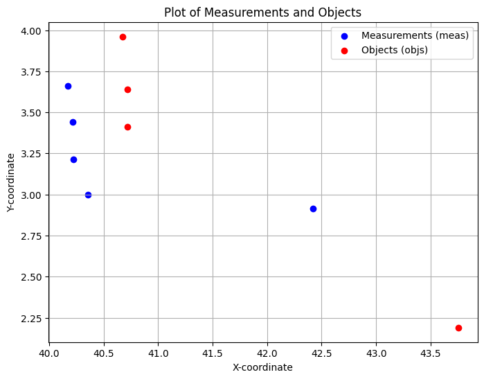
The problem shown here is an artificial one. Five measurements are given as two-dimensional positions. We got as well four object positions in 2D. The one-to-one association of measurements with objects might appear ambiguous for the human eye. One measurement can be associated to exacly one object or is clutter/new born. One object can be associated to exactly one measurement or is misdetected. Using just the euclidean distance might lead to a violation of these constraints.

Includes

import numpy as np
import torch
import random
import os
import matplotlib.pyplot as plt
import sys

Measurements and Objects

# Measurements
points = torch.tensor([
    [40.1732, 3.66123],
    [40.2158, 3.43958],
    [40.2211, 3.21301],
    [40.3561, 2.99893],
    [42.4198, 2.91224],
])

points = torch.t(points)
meas_x = points[0,:]
meas_y = points[1,:]

# Objects
objs = torch.tensor([
    [40.7211, 3.41301],
    [40.7158, 3.63958],
    [40.6732, 3.96123],
    [43.7526, 2.19003]
])

objs = torch.t(objs)
objs_x = objs[0,:]
objs_y = objs[1,:]

# plot the measurements meas and the objects

plt.figure(figsize=(8, 6)) # Create a new figure for clarity
plt.scatter(meas_x.numpy(), meas_y.numpy(), label='Measurements (meas)', color='blue')
plt.scatter(objs_x.numpy(), objs_y.numpy(), label='Objects (objs)', color='red')
plt.xlabel('X-coordinate')
plt.ylabel('Y-coordinate')
plt.title('Plot of Measurements and Objects')
plt.legend()
plt.grid(True)
plt.show()

Shuffle the measurements and object

# Get the number of measurements and objects
num_measurements = meas_x.shape[0]
num_objects = objs_x.shape[0]

# Create shuffled indices for measurements and objects
shuffled_meas_indices = torch.randperm(num_measurements)
shuffled_objs_indices = torch.randperm(num_objects)

# Shuffle the measurements and objects using the shuffled indices
shuffled_meas_x = meas_x[shuffled_meas_indices]
shuffled_meas_y = meas_y[shuffled_meas_indices]

shuffled_objs_x = objs_x[shuffled_objs_indices]
shuffled_objs_y = objs_y[shuffled_objs_indices]

Compute a distance matrix using the shuffeled measurements

# Reshape shuffled measurements and objects for broadcasting
shuffled_meas = torch.stack((shuffled_meas_x, shuffled_meas_y), dim=1)
shuffled_objs = torch.stack((shuffled_objs_x, shuffled_objs_y), dim=1)

shuffled_meas = torch.stack((meas_x, meas_y), dim=1)
shuffled_objs = torch.stack((objs_x, objs_y), dim=1)

# Compute the squared difference in x and y coordinates
diff_x = shuffled_meas[:, None, 0] - shuffled_objs[None, :, 0]
diff_y = shuffled_meas[:, None, 1] - shuffled_objs[None, :, 1]


# Compute the squared Euclidean distance
dist_sq = diff_x**2 + diff_y**2

# Take the square root to get the Euclidean distance matrix
#distance_matrix = -torch.sqrt(dist_sq)
distance_matrix = -dist_sq

# distance_matrix = torch.cat((distance_matrix, torch.ones(num_measurements, 1) * -2.), dim=1) # column for clutter
# distance_matrix = torch.cat((distance_matrix, torch.ones(1, num_objects + 1) * -2.), dim=0) # row for misdetections

print("Distance Matrix:")
distance_matrix

Distance Matrix:





tensor([[ -0.3618,  -0.2949,  -0.3400, -14.9766],
        [ -0.2560,  -0.2900,  -0.4813, -14.0703],
        [ -0.2900,  -0.4267,  -0.7642, -13.5180],
        [ -0.3047,  -0.5398,  -1.0266, -12.1906],
        [ -3.1364,  -3.4326,  -4.1510,  -2.2979]])

MASDA - iteration and compute the belief

# both beta and rho matrices are initialized with a large positive value (1e+3)
# for all their elements. In the context of the Max-Sum algorithm, where
# messages represent scores or preferences, initializing with a large positive
# value like this often serves as a 'neutral' or 'uninformative' starting point.
# It essentially means that, initially, there is no strong preference for any
# particular association (or non-association) based on prior messages.
beta = torch.ones(distance_matrix.shape) * 1e+3
rho = torch.ones(distance_matrix.shape) * 1e+3
n_meas_assoc = distance_matrix.shape[0]
n_obj_assoc = distance_matrix.shape[1]

# Define the constant costs/scores for misdetection and clutter.
# These represent the prior belief or preference for an object to be misdetected
# or a measurement to be clutter/newly born.
misdetection = -1.0
clutter = misdetection


# print("n_objs:", n_obj_assoc)
# print("n_points:", n_meas_assoc)
# print("n_objs:", num_objects)
# print("n_points:", num_measurements)

# Damping factor to stabilize message updates, especially in loopy graphs.
# A value of 0.0 means no damping (messages are fully replaced each iteration).
# A value closer to 1.0 would mean messages change slowly (weighted average of old and new).
damping = 0.0

# Initialize belief matrix. It will store the final scores for each possible assignment,
# including clutter and misdetection cases.
belief = torch.ones((n_meas_assoc + 1, n_obj_assoc + 1)) * misdetection

# Function to compute the final beliefs after message passing.
# The belief for each assignment (measurement i to object j, clutter, or misdetection)
# is the sum of relevant incoming messages and the similarity score.
def compute_belief():
    # Iterate through each measurement to calculate its association beliefs
    for i in range(num_measurements):
        # Mask for object-specific calculations: ensures we don't consider
        # the current object's own message when calculating max for alpha.
        # This large value effectively 'removes' the current element from max operations
        # by making it so large that it will never be selected.
        mask_meas = torch.zeros(n_meas_assoc)
        mask_meas[i] = 1.e+20

        # Calculate beliefs for measurement-to-object associations
        for j in range(num_objects):
            # Mask for measurement-specific calculations: similar to mask_meas but for beta.
            mask_obj = torch.zeros(n_obj_assoc)
            mask_obj[j] = 1.e+20
            # eta_ij = -max_{k!=j} beta_ik (message from I_i to c_ij)
            # It represents the penalty if measurement 'i' were associated with 'j',
            # considering alternatives to 'j'.
            eta = - torch.max(torch.max(beta[i,:] - mask_obj), torch.tensor(clutter))
            # alpha_ij = -max_{k!=i} rho_kj (message from E_j to c_ij)
            # It represents the penalty if object 'j' were associated with 'i',
            # considering alternatives to 'i'.
            alpha = - torch.max(torch.max(rho[:,j] - mask_meas), torch.tensor(clutter))
            # The belief for associating measurement 'i' with object 'j' is the sum of
            # these two messages and the direct similarity score.
            belief[i,j] = eta + alpha + distance_matrix[i,j]

    # Calculate beliefs for measurements being clutter (new born object)
    for i in range(num_measurements):
        j = num_objects # This represents the 'clutter' column
        # eta_i,n+1 = -max_{k} beta_ik (message from I_i to e_i)
        # It represents the penalty if measurement 'i' is clutter, considering all object alternatives.
        eta = - torch.max(beta[i,:])
        # Belief for measurement 'i' being clutter is this message plus the clutter cost.
        belief[i,j] = eta + clutter

    # Calculate beliefs for objects being misdetected
    for j in range(num_objects):
        i = num_measurements # This represents the 'misdetection' row
        # alpha_m+1,j = -max_{k} rho_kj (message from E_j to d_j)
        # It represents the penalty if object 'j' is misdetected, considering all measurement alternatives.
        alpha = - torch.max(rho[:,j])
        # Belief for object 'j' being misdetected is this message plus the misdetection cost.
        belief[i,j] = alpha + misdetection

    # print("Belief:\n", belief)
    # print(torch.sum(belief))

# Main message passing loop
for iter in range(6):
   # Update beta messages (variable to factor I_i)
   for i in range(num_measurements):
        # Create a mask to exclude the current measurement's own message when calculating
        # the maximum over rho_kj in the beta update.
        mask = torch.zeros(n_meas_assoc)
        mask[i] = 1.e+20 # Large value to ensure it's not chosen by torch.max

        for j in range(num_objects):
            # Beta update: beta_ij = s(i,j) - max_{k!=i} rho_kj
            # max_val here computes max_{k!=i} rho_kj or clutter
            max_val = torch.max(torch.max(rho[:,j] - mask), torch.tensor(clutter))
            # Apply damping to the message update
            beta[i,j] = beta[i,j] * damping + (distance_matrix[i,j] - max_val) * (1. - damping)

   # Update rho messages (variable to factor E_j)
   for j in range(num_objects):
        # Create a mask to exclude the current object's own message when calculating
        # the maximum over beta_ik in the rho update.
        mask = torch.zeros(n_obj_assoc)
        mask[j] = 1.e+20 # Large value to ensure it's not chosen by torch.max

        for i in range(num_measurements):
            # Rho update: rho_ij = s(i,j) - max_{k!=j} beta_ik
            # max_val here computes max_{k!=j} beta_ik or misdetection
            max_val = torch.max(torch.max(beta[i,:] - mask), torch.tensor(misdetection))
            # Apply damping to the message update
            rho[i,j] = rho[i,j] * damping + (distance_matrix[i,j] - max_val) * (1. - damping)

   # print rho and beta
   # print("beta: ", beta)
   # print("rho: ", rho)

# Recompute beliefs after message passing
compute_belief()
# print(belief)

Plot the association

# get the maximum index from beta and plot the point association using this information

beta_misdetection = torch.cat((beta, torch.ones(num_measurements, 1) * misdetection), dim=1) # column for clutter
# distance_matrix = torch.cat((distance_matrix, torch.ones(1, num_objects + 1) * -2.), dim=0) # row for misdetections

beta_misdetection = belief
# print(beta_misdetection)

# Get the index of the maximum value in beta
max_beta_index = torch.argmax(beta_misdetection,1)
# print(max_beta_index)

# Convert the linear index to row and column indices
row_index = range(num_measurements)
col_index = max_beta_index

# print(f"Maximum value of beta is at index: ({row_index}, {col_index})")

# Extract the associated points from the shuffled measurements and objects
associated_measurement = shuffled_meas[row_index]

# print(f"Associated Measurement Point:\n{associated_measurement.numpy()}")
# print(f"Associated Object Point:\n{associated_object.numpy()}")

# Plot the associated points and a line connecting them
plt.figure(figsize=(8, 6))
plt.scatter(shuffled_meas_x.numpy(), shuffled_meas_y.numpy(), label='Shuffled Measurements', color='blue', alpha=0.5)
plt.scatter(shuffled_objs_x.numpy(), shuffled_objs_y.numpy(), label='Shuffled Objects', color='red', alpha=0.5)
for i in range(num_measurements):
    if max_beta_index[i] < num_objects:
        plt.plot([shuffled_meas[i][0].numpy(), shuffled_objs[max_beta_index[i]][0].numpy()],
            [shuffled_meas[i][1].numpy(), shuffled_objs[max_beta_index[i]][1].numpy()],
                color='green', linestyle='--', label='Association')

plt.xlabel('X-coordinate')
plt.ylabel('Y-coordinate')
plt.title('Point Association based on Maximum Beta')
plt.legend()
plt.grid(True)
plt.show()

Discussion

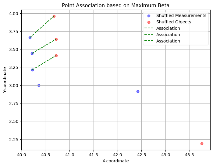
A sensible association hypothesis was found by the algorithm, associating the top left measurements with the top left objects. The other two measurements were not associated, as there is no other object available in their vicinity. Thus, the bottom right object remains undetected.

The computation of the similarities is too simplistic here to be considered a real-world example. One would incorporate uncertainties. Further, in a scenario with objects and measurements streaming from radar or a lidar, one would incorporate detection probabilities and clutter probabilities based on some functions that model the capabilities of the sensor and the environmental constraints.