In Faster Data Association with Max-Sum Loopy Belief Propagation (MASDA) I derived MASDA for the tracking problem: associate measurements with objects, allowing for clutter and misdetection. Stereo matching has the same structure, so this post applies MASDA there — to the dense problem, a disparity for every pixel — and measures what it gains.
The formulation runs on sparse matrices. Each pixel offers only its two best disparity candidates out of the aggregated cost volume, so the association graph carries two edges per pixel instead of a \(W \times W\) matrix per row, and every result below depends on that representation twice over: it is what makes the exact comparison feasible, and it is what makes the solver fast.
Part 2 takes this formulation into C++ on a Jetson TX2 and measures it against SGM; Part 3 makes it real-time on the TX2’s GPU, bit-identically.
Every technical term this series uses — from factor graphs to CUDA warps — is defined in the glossary for this series, with links to the original work. Terms link there on first use, in all three parts.
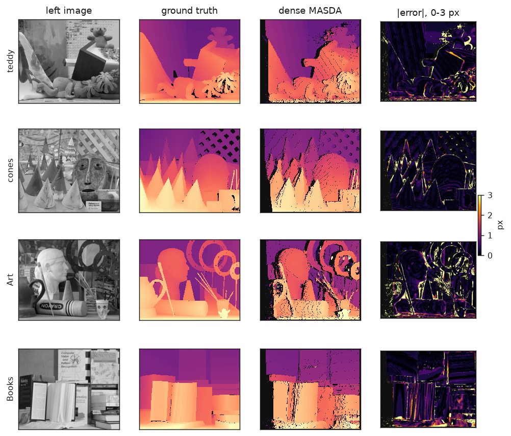
Results, briefly — pooled over eight Middlebury scenes with structured-light ground truth, roughly 1.3 million answers:
- The one-to-one constraint is worth +11.5 points of precision over winner-take-all on identical scores: 0.890 against 0.775, while keeping 95% of WTA’s correct answers. Per scene the gain is 8–13 points, largest where the texture is worst.
- The constraint is what pays, not the message passing. Applying the same greedy one-to-one claim to each pixel’s top-1 score — no messages at all — reaches 0.890. Full MASDA reaches 0.883, trading 0.8 points of precision for 6,333 more answers. The engineered matcher in Part 2 reproduces this independently, in different code on a harder benchmark.
- Loopy max-sum matches the exact assignment optimum on precision where the exact optimum is computable: per-row Jonker-Volgenant reaches 0.914 and 0.941 on Teddy and Cones; MASDA reaches 0.915 and 0.942.
- It does that from two message-passing iterations, sitting 0.8% short of the optimal objective with 1.6% of rows exactly optimal. Thirty iterations close the objective gap to 0.08% and make 47–69% of rows optimal — and return no extra precision at all. The decision stabilises an order of magnitude before the objective does, which is the single most useful thing I learned here.
- The representation decides the speed. The same messages on dense per-row matrices: 7.2 s per frame. On sparse matrices: 0.38 s — 19× — and 20× faster than compiled per-row Jonker-Volgenant. The engineered C++ descendant of this NumPy study solves the same frames in ~11 ms, and the full GPU pipeline of Part 3 runs at 28.9 ms per frame end to end.
Everything is regenerable: article/dense_sparse_matrices.py produces every
number in this post from the shipping binary’s own cost volume, so the NumPy
study and the production pipeline are measured on identical scores.
1. Dense stereo as a data association problem
In tracking, data association puts measurements \(i \in \{1 \dots m\}\) with objects \(j \in \{1 \dots n\}\), at most one each way, with the option of calling a measurement clutter or an object misdetected.
For stereo, substitute the nouns — per rectified image row. Pixels in the left row are measurements, pixels in the right row are objects. At most one association each way, because one surface point produces one projection per image. A left pixel whose surface is occluded in the right view has no partner at all, which is clutter (\(\lambda\)). A right pixel whose surface is hidden from the left camera is a misdetection (\(\gamma\)). Occlusion is not a small correction: on these scenes it affects 10–20% of pixels, and a formulation that assumes every pixel is matchable is wrong exactly at the depth discontinuities where stereo is hardest.
What stereo adds is geometry. The pair is rectified, so correspondences lie on the same image row and disparity \(d = x_L - x_R\) is positive and bounded. Each row is an independent association problem — which makes the whole thing parallel, and later, a GPU workload.
1.1 Factor graph
Same as the tracking case, on the same factor graph: binary association variables \(c_{ij}\), clutter indicators \(e_i\), misdetection indicators \(\delta_j\), similarity factors \(S_{ij}\), clutter factors \(\Lambda_i\), misdetection factors \(\Gamma_j\), and the exclusivity constraints \(I_i\) and \(E_j\).
The graph is loopy. Every \(c_{ij}\) sits in both an \(I_i\) and an \(E_j\) constraint, so there are four-cycles everywhere. Hence loopy belief propagation, and hence no convergence guarantee.
1.2 Messages
The two message directions are unchanged:
\[\begin{aligned} \beta_{ij} &= s(i,j) - \max_{k \neq i} \rho_{kj} \\ \rho_{ij} &= s(i,j) - \max_{k \neq j} \beta_{ik} \end{aligned}\]with the non-association options competing inside those maxima:
\[\begin{aligned} \rho_{ij} &= s(i,j) - \max\!\left(\lambda,\; \max_{k \neq j} \beta_{ik}\right) \\ \beta_{ij} &= s(i,j) - \max\!\left(\gamma,\; \max_{k \neq i} \rho_{kj}\right) \end{aligned}\]\(\rho_{ij}\) reads as: how good is associating \(i\) with \(j\), after subtracting the best thing \(i\) could do instead, where “instead” includes being called clutter. \(\beta_{ij}\) is the same from the object side.
Damping on both:
\[x^{(t+1)} \leftarrow (1-\eta)\, x_{\text{target}} + \eta\, x^{(t)}\]The belief combines both directions,
\[b_{ij} = \alpha_{ij} + \eta_{ij} + s_{ij}\]and since \(\beta_{ij} = s_{ij} + \alpha_{ij}\) and \(\rho_{ij} = s_{ij} + \eta_{ij}\), in code this is
\[b_{ij} = \beta_{ij} + \rho_{ij} - s_{ij}\]Both maxima exclude one element, so caching the largest and second-largest per row and column makes “max excluding \(j\)” constant time. An iteration is then two linear passes over the edges:
\[O(T \cdot E), \qquad E = |\{(i,j) : \text{candidate}\}|\]In the dense formulation, \(E = 2\) per pixel — the two best candidates out of the aggregated volume — so a 450-pixel row carries ~900 edges instead of the ~200,000 cells of its full matrix. Why two is the right number is measured in Part 2: keeping eight candidates per pixel is measurably worse than keeping two, because the extra candidates are noise, and the solver has to weigh them against the real ones.
1.3 The score
Descriptors are the Census transform over a
\(7 \times 7\) window: one bit per
neighbour, set when the neighbour is darker than the centre. 48 bits fit a
uint64, so the distance is a single
popcount, and Census is invariant to
monotonic intensity mappings, which absorbs gain and offset differences between
two real sensors.
Two unrelated Census descriptors agree on half their bits by chance, so scaling the Hamming distance \(h\) around that point gives a score with a usable zero: \(+1\) perfect, \(0\) chance. On this scale \(\lambda = \gamma = -0.1\) means “reject anything worse than a tenth of the way from chance to perfect”, which is easier to reason about than a tuned constant.
One pixel’s Census comparison quantises to only 49 levels, which is not enough signal per pixel. The score MASDA actually consumes is aggregated over an edge-aware support region — an O(N) recursive filter that stops at intensity edges — so each candidate’s score summarises a neighbourhood while respecting depth boundaries. The aggregation machinery, and the measurements behind each of its choices, are Part 2’s subject; here it is the given: the sparse candidate matrix is built from the aggregated volume of the shipping implementation, so this study and the production pipeline score identical evidence.
2. Ground truth
The matcher is measured on Teddy and Cones from the Middlebury 2003 stereo set, and on the six Middlebury 2005 scenes: Art, Books, Dolls, Laundry, Moebius and Reindeer, at third size. They are rectified, and they ship structured-light ground truth at quarter-pixel resolution with a few percent of pixels marked unknown. The dataset page states: “We grant permission to use and publish all images and disparity maps on this website.”
D. Scharstein and R. Szeliski (2003). High-accuracy stereo depth maps using structured light. CVPR, 195-202. doi:10.1109/CVPR.2003.1211354
D. Scharstein and C. Pal (2007). Learning conditional random fields for stereo. CVPR. doi:10.1109/CVPR.2007.383191
The 2005 two-view archives ship no documented disparity scale, so the factor of 3 is established rather than assumed: for a pixel at \(x\) in the left view with true disparity \(t\), the right view’s disparity map at \(x - t\) must also read \(t\). That identity holds to a median of 0.000 px at a scale of 3 and fails at every other integer, and it involves no matcher, so it cannot flatter the results.
Middlebury marks unknown disparity as zero rather than shipping a separate visibility mask, so an answer landing on an unknown pixel has no correct value to be compared against. Those are excluded from precision rather than scored as wrong, which would charge the matcher for holes in the dataset.
3. Implementation
Both updates need the same primitive: for every candidate, the best of the alternatives it is competing against — the maximum along its row or column with itself left out. Computed naively that is a scan per entry and the iteration is quadratic. It is two reductions instead, because a line has only one argmax:
def top2_excluding(A, axis):
    """For every entry, the max of its row (axis=1) or column (axis=0)
    EXCLUDING that entry itself.

    The line's largest value is the answer for every entry except the argmax
    itself, which gets the second largest. Two reductions, no per-entry scan --
    this is what makes an iteration linear in the number of candidates.
    """
    i1 = np.expand_dims(np.argmax(A, axis=axis), axis)
    m1 = np.take_along_axis(A, i1, axis)              # the largest
    B = A.copy()
    np.put_along_axis(B, i1, -np.inf, axis)
    m2 = np.max(B, axis=axis, keepdims=True)          # the second largest
    out = np.broadcast_to(m1, A.shape).copy()
    np.put_along_axis(out, i1, m2, axis)              # only the argmax differs
    return out
Ties and dead entries are the cases to get right, and this form handles both: the
substitution is by index, so two equal maxima do not both get demoted, and a line
of -inf returns -inf. Checked against a brute-force scan over 6000 random
matrices with a deliberately small value range, no disagreements.
The solver, in the notation above — the dense-matrix reference version:
def masda(S, lam=-0.1, gam=-0.1, iters=30, damping=0.4, eps=1e-5):
    finite = np.isfinite(S)
    beta = np.where(finite, 0.0, -np.inf)
    rho  = beta.copy()

    for it in range(iters):
        # rho: a row's other options, or calling this measurement clutter
        comp = np.maximum(lam, top2_excluding(np.where(finite, beta, -np.inf), 1))
        new_rho = np.where(finite, (1 - damping) * (S - comp) + damping * rho, -np.inf)

        # beta: a column's other options, or calling this object misdetected
        comp = np.maximum(gam, top2_excluding(np.where(finite, new_rho, -np.inf), 0))
        new_beta = np.where(finite, (1 - damping) * (S - comp) + damping * beta, -np.inf)

        delta = max(np.nanmax(np.abs(new_rho - rho)),
                    np.nanmax(np.abs(new_beta - beta)))
        rho, beta = new_rho, new_beta
        if delta < eps:
            break

    belief = np.where(finite, beta + rho - S, -np.inf)
    return decide(S, belief, lam)
3.1 Reading out the answer
I got this wrong on the first attempt, and the mistake follows directly from the theory, so it is worth walking through.
I gated acceptance on \(b_{ij} > 0\). On problems with exactly tied candidates that returned zero matches, on problems whose optimum matched everything.
The belief measures an edge’s advantage over its competitors. When nothing has an advantage, every belief is \(\le 0\). That is also the condition under which the LP relaxation has no unique optimum, and uniqueness is exactly what Bayati, Shah and Sharma require for max-product to be correct on bipartite matching. So the degenerate case is not an edge case to patch around; it is where the guarantee stops. Section 4 measures how often that happens on dense rows, and it is often.
Bayati, M., Shah, D., & Sharma, M. (2008). Max-Product for Maximum Weight Matching: Convergence, Correctness, and LP Duality. IEEE Transactions on Information Theory, 54(3), 1241-1251. doi:10.1109/TIT.2007.915695
Two questions were tangled together:
| question | answered by |
|---|---|
| which candidate? | the belief \(b_{ij}\), as an ordering. Its sign means nothing. |
| associate at all? | \(s(i,j)\) against \(\lambda\), which is what \(\lambda\) is for. |
So: order by belief, decide by \(\lambda\), require row and column to agree, then fill in greedily by belief over what is left. The greedy fill is not cosmetic: under near-ties every row’s best belief points at the same column, so requiring mutual agreement commits exactly one pair, and every greedily accepted edge has \(s > \lambda\) and two free endpoints, so it raises the objective.
3.2 The sparse-matrix form — this is the design, not an optimisation
Put the messages on the edges. The only awkward part is that both updates need \(\max_{k \neq j}\) over a row or column, which is quadratic in row length if done directly. Three segment reductions answer it exactly in \(O(E)\):
def _seg_max_excluding(vals, idx, n):
    """Per-segment max with each element's own contribution removed, in O(E)."""
    m1 = np.full(n, -np.inf)
    np.maximum.at(m1, idx, vals)          # segment max
    at_max = vals >= m1[idx]              # m1 is the max, so >= means ==
    cnt = np.zeros(n, np.int64)
    np.add.at(cnt, idx[at_max], 1)        # how many attain it
    m2 = np.full(n, -np.inf)
    below = ~at_max
    if below.any():
        np.maximum.at(m2, idx[below], vals[below])   # max strictly below
    second = np.where(cnt > 1, m1, m2)
    return np.where(at_max, second[idx], m1[idx])
Three cases: an element below the max sees the max; an element at the max also sees the max, provided something else attains it; otherwise it sees the runner-up. Ties need handling rather than ignoring, since near-ties are the case of interest.
The solver is then five lines per iteration:
def masda_sparse(ei, ej, se, m, n, lam=-0.1, gam=-0.1, iters=30, damping=0.4):
    beta = np.zeros(len(se)); rho = np.zeros(len(se))
    for _ in range(iters):
        comp = np.maximum(lam, _seg_max_excluding(beta, ei, m))
        new_rho  = (1 - damping) * (se - comp) + damping * rho
        comp = np.maximum(gam, _seg_max_excluding(new_rho, ej, n))
        new_beta = (1 - damping) * (se - comp) + damping * beta
        rho, beta = new_rho, new_beta
    belief = beta + rho - se
    ...
Same messages, same damping, same belief, same decision rule as the dense-matrix version. Only the representation differs — and section 5 shows that difference is a factor of 62 on this problem, before any compiled code.
A note on damping: undamped max-sum on heavily tied problems does not settle; the largest message change plateaus instead of decaying. Damping of 0.3–0.5 stabilises it, and solution quality is flat across that range. Message convergence is not the property you need anyway — the decision stabilises long before the messages do, and section 4.3 measures how much sooner: fifteen times sooner, on these scenes.
4. Results against ground truth
\(\lambda = \gamma = -0.1\), two iterations — the shipping configuration — damping 0.4, candidates = top-2 per pixel from the aggregated volume, tolerance 1 px, unknown ground truth excluded. (Section 4.3 measures what the other 28 iterations would buy, which is nothing.) Three solvers on identical scores: winner-take-all (argmax over the full volume — no uniqueness), MASDA on the sparse candidate matrix, and per-row exact assignment (Jonker-Volgenant with explicit \(\lambda\)/\(\gamma\) slots, so non-association is a real option for it too).
4.1 What uniqueness is worth
Pooled over all eight scenes — about 1.3 million answered pixels per method:
| method | correct | wrong | precision |
|---|---|---|---|
| winner-take-all — argmax, no uniqueness | 1,006,811 | 292,281 | 0.775 |
| greedy uniqueness on the top-1 score, no messages | 961,427 | 118,616 | 0.890 |
| MASDA, sparse matrices, 2 iterations | 967,760 | 128,683 | 0.883 |
+11.5 points of precision for the one-to-one constraint, at the cost of 4.5% of the correct answers. WTA answers everywhere and is wrong more than twice as often.
The middle row is the one that decides where the credit belongs, and it is worth being precise about. It applies the same greedy one-to-one claim MASDA’s decode uses — best score first, each right pixel claimable once — to each pixel’s top-1 score, with no message passing at all. The constraint delivers the entire gain. The message passing costs 0.8 points of precision and returns 6,333 more correct answers, which is the same trade the margin gate offers for free.
That is not the reading I expected when I built this, and it is reproduced independently in Part 2 by the engineered C++ matcher, in a different codebase, on a different benchmark, at a different tolerance: disabling the message passing there measures better and saves twelve milliseconds of CPU per frame. Two measurements that share no code agree on the shape.
What the messages do earn is visible in the next two sections: they get closer to the exact assignment objective, and they do it while remaining an approximation. The objective is simply not the quantity a consumer experiences — which is the finding of section 4.2, arriving early.
Per scene, WTA against MASDA:
| scene | WTA | MASDA | Δ |
|---|---|---|---|
| Art | 0.700 | 0.830 | +13.0 |
| Books | 0.796 | 0.901 | +10.5 |
| Dolls | 0.810 | 0.915 | +10.5 |
| Laundry | 0.661 | 0.777 | +11.6 |
| Moebius | 0.788 | 0.878 | +9.0 |
| Reindeer | 0.769 | 0.905 | +13.6 |
| Cones | 0.859 | 0.942 | +8.3 |
| Teddy | 0.826 | 0.911 | +8.5 |
The gain is largest on the worst scenes (Art, Laundry, Reindeer), which is the right shape: where the descriptor evidence is weakest, mutual exclusivity has the most to contribute. The constraint pays in proportion to the ambiguity, and here that is measured over 1.3 million answers.
For the full engineered pipeline (the C++ implementation with its margin gate, which trades a little coverage for precision), Part 2 measures 24.5% bad-1.0 at 79.6% coverage on the fifteen Middlebury v3 training scenes, against the benchmark’s own SGM reference at 29.1% and 90.2% — a lower error rate over the pixels it answers, ten points fewer of them, and a curve that runs below SGM’s where the two overlap. On these eight 2003/2005 scenes at native resolution it measures 9.8% against OpenCV SGM’s 10.9%. Both are real; the harder benchmark and the looser one disagree about the ordering, and Part 2 shows why.
4.2 Against the exact optimum
Per-row Jonker-Volgenant is feasible on the sparse problem (900 edges per row), so the exact comparison covers every row of Teddy and Cones:
| scene | method | correct | precision | objective ratio | rows at exact optimum |
|---|---|---|---|---|---|
| Teddy | MASDA, 2 iters | 130,413 | 0.915 | 0.9918 | 6 / 369 |
| Teddy | MASDA, 30 iters | 131,152 | 0.914 | 0.9992 | 175 / 369 |
| Teddy | JV (exact) | 131,210 | 0.914 | 1 | — |
| Cones | MASDA, 2 iters | 130,956 | 0.942 | 0.9939 | 0 / 369 |
| Cones | MASDA, 30 iters | 131,443 | 0.941 | 0.9996 | 253 / 369 |
| Cones | JV (exact) | 131,482 | 0.941 | 1 | — |
Three readings, and the third is the one I did not expect.
Precision is indistinguishable from exact. 0.915 against 0.914, 0.942 against 0.941. The exact solver finds a few hundred more correct answers out of 131 thousand and is fractionally less precise, because it answers more often. Whatever approximation error loopy max-sum commits here, it is not made of wrong disparities.
It is genuinely an approximation. The objective ratio against JV never reaches 1: 0.9918 at the shipping setting, and even at thirty iterations MASDA reaches the exact optimum on only 47% and 69% of rows. The difference is ties. An aggregated Census volume quantises to few enough levels that exactly tied candidates are everywhere, so the LP-uniqueness condition of the Bayati-Shah-Sharma guarantee fails routinely.
And the gap costs nothing. Two iterations sit 0.8% short of the optimal objective with 1.6% of rows optimal; thirty iterations close that to 0.08% and 47% — and return no extra precision whatsoever. The objective is a proxy, and this is the cleanest evidence I have that it is a loose one: an 0.8% objective deficit and a 30× shortfall in exactly-solved rows are invisible in the only quantity a consumer experiences.
4.3 Two iterations against thirty
Since the shipping implementation runs two iterations and this study originally ran thirty, the difference is worth its own table. Pooled over all eight scenes:
| iterations | correct | precision | objective ratio (Teddy) | rows optimal |
|---|---|---|---|---|
| 2 (shipping) | 242,824 | 0.884 | 0.9918 | 6 / 369 |
| 30 | 243,589 | 0.880 | 0.9992 | 175 / 369 |
Fifteen times the message passing buys 0.3% more correct answers, 0.4 points less precision, and a solve four times slower. The extra iterations move marginal candidates from “not answered” to “answered”, and those marginal candidates are wrong slightly more often than the population average — so the objective improves while precision does not.
This is the quantitative form of a claim section 3.2 makes qualitatively: message convergence is not the property you need. The messages are still moving at iteration thirty; the decision stopped moving around iteration two. Every number elsewhere in this article is therefore reported at the shipping setting, and I would treat any belief-propagation matcher quoting an iteration count without this comparison with suspicion — including my own earlier version of this page.
5. Speed: the representation decides it
The complexity argument is \(O(T \cdot E)\) against Jonker-Volgenant’s \(O(N^3)\). Written the obvious way — messages in a per-row \(W \times W\) matrix padded with \(-\infty\) — the argument buys nothing: with two real candidates per pixel, more than 99% of the arithmetic lands on \(-\infty\) cells.
One frame of Teddy (369 rows, 326,565 edges), same solvers, same answers:
| representation | 2 iterations | 30 iterations |
|---|---|---|
| dense per-row matrices | 7.22 s | 96.9 s |
| sparse matrices (edge list) | 0.38 s | 1.57 s |
| per-row JV (scipy, compiled) | 7.6 s | 10.0 s |
At the shipping setting the sparse-matrix solver is 19× faster than the same mathematics on dense matrices and 20× faster than compiled exact assignment — from interpreted NumPy. (Jonker-Volgenant does not depend on the iteration count at all; its two entries differ only by measurement noise on a shared desktop, which is a useful reminder of how much precision to read into any single row of this table.) These are study numbers, not production numbers: the identical algorithm in C++ (Part 2) solves a frame in ~11 ms on a desktop and ~23 ms on the Jetson TX2’s ARM cores, and the full GPU pipeline (Part 3) — cost volume, aggregation and solve together — runs at 28.9 ms per frame at 848×480, bit-identical to the C++ output. Five orders of magnitude between the first table’s first row and the shipping pipeline, and not one change to the messages: representation, then engineering.
The actual claim, then: MASDA’s cost is linear in the number of plausible associations, and the aggregated volume plus geometry cuts a \(W \times W\) row problem to two candidates per pixel. Only a representation that exploits that sees any benefit. This also reframes the comparison with an exact solver: it is not about accuracy — section 4.2 shows JV is exactly as good — it is that MASDA is anytime, incremental, and accepts factors that destroy the assignment structure, where a LAP solver cannot follow.
6. Can MASDA express the ordering constraint?
Scanline stereo methods use the ordering constraint: matches along a scanline should not cross. This is the one thing scanline dynamic programming gets for free and a plain assignment formulation does not, so it is the standing objection to using MASDA for dense stereo. It can be added as a factor, the derivation is tidier than I expected, and on the dense problem it costs more than it returns.
Two associations \((i,j)\) and \((i',j')\) cross iff \((x_i - x_{i'})(x_j - x_{j'}) < 0\). A matching is order-preserving exactly when no two of its pairs cross, so ordering decomposes into pairwise factors with no higher-order term. That is what makes it tractable.
Take \(\psi(c_e, c_f) = -\kappa\) when both edges are on and crossing, else 0. For a pairwise factor between binary variables only the difference of the outgoing message matters, and with \(\mu_f = m_f(1) - m_f(0)\):
\[\Delta_{\psi \to e} = \max(0, \mu_f - \kappa) - \max(0, \mu_f) = -\operatorname{clamp}(\mu_f,\, 0,\, \kappa)\]The ordering message is the conflicting edge’s own preference, clamped and negated. One scalar, constant time. I checked it against brute-force max-sum over 20000 random cases; agreement is 4×10⁻¹⁶.
It composes with the sparse-matrix form without touching it. Because these messages are additive on the edge they fold into the score: writing \(o_e = -\sum_{f \in X(e)} \operatorname{clamp}(b_f, 0, \kappa)\) for the summed ordering pressure, the updates are the same two segment reductions of section 3.2 with \(s + o\) substituted for \(s\). No new message type, no change to the solver’s structure. This is the property that makes MASDA worth preferring over an exact assignment solver, which cannot follow here at all.
It does not make the problem smaller, and the reason is worth stating because the opposite is the natural guess. Ordering constrains pairs of associations, not single ones: no individual \((i,j)\) becomes illegal, it is only forbidden in combination with some other pair. The edge set — the thing that makes the matrix sparse — is therefore untouched, and what the factor contributes is a per-edge penalty folded into the score. The matrix keeps its shape; the numbers in it change.
The guess is right for a different algorithm. Scanline dynamic programming commits matches left to right, so once \((i,j)\) is fixed every crossing candidate for every later pixel is gone and the remaining search really does shrink — that is what “ordering is free in DP” means. MASDA commits nothing until the decode and settles the whole row jointly, so it has to represent the constraint rather than exploit it. Representing it costs about 2400 crossing pairs against 885 edges on a dense row, which is the 3:1 that the measurement turns into 5–7× the solve.
What that buys is a constraint DP cannot have: a soft one. \(\kappa\) stays finite. Thin foreground objects genuinely violate ordering, and a hard constraint would delete them — the standard failure of DP-based scanline methods, which is why they need forbidden-move exceptions.
6.1 Measured, dense: it works, and it costs more than it returns
Eight scenes, every fourth row, paired against the same rows with the factor off, \(\kappa = 0.3\), damping raised to 0.6 because the ordering factors add loops the bipartite convergence result does not cover:
| scene | precision, off | on | Δ | crossings retained |
|---|---|---|---|---|
| Art | 0.825 | 0.828 | +0.3 | 0.67× |
| Books | 0.897 | 0.901 | +0.4 | 0.33× |
| Dolls | 0.910 | 0.911 | +0.1 | 0.56× |
| Laundry | 0.771 | 0.780 | +0.9 | 0.47× |
| Moebius | 0.874 | 0.879 | +0.5 | 0.65× |
| Reindeer | 0.900 | 0.907 | +0.7 | 0.60× |
| Cones | 0.941 | 0.943 | +0.2 | 0.59× |
| Teddy | 0.912 | 0.915 | +0.3 | 0.47× |
The factor does exactly what the derivation says: it removes about half the crossings (0.54× on average, never worse than 0.67×) and improves precision on all eight scenes — mean +0.43 points, standard error 0.094, and unanimous, which matters more than the \(t\)-statistic on eight scenes. The gain is largest where the scene is worst (Laundry +0.9 at precision 0.771, Reindeer +0.7), the same shape uniqueness itself shows in section 4.1.
And it is not worth switching on, for a reason that is specific to the dense formulation: the band is the whole row. Every pixel is a node, so a row carries ~885 edges and ~2400 crossing pairs — they outnumber edges by nearly 3:1, and the \(O(E_r^2)\) enumeration that is free on a handful of nodes becomes the largest item on the board. Enumerating and reducing over 600,000 of them per scene is 5–7× the entire solve, to buy 0.4 points of precision — against a factor of 62 that the sparse-matrix representation buys for free, and 40 more correct answers out of 243,000.
The \(\kappa\) sweep says the same thing from another direction: 0.1, 0.3 and 0.8 all land within 0.003 of one another on precision and within 1% on crossings retained. The factor saturates immediately — it is not being tuned into usefulness, it is doing all it can do and that is a small thing.
So: ordering is expressible inside the existing closed form, and on the dense problem it is a real but poor trade. The \(O(E_r \log E_r)\) Fenwick-tree construction is a precondition here rather than an optimisation, and even at that price the 0.4-point return does not obviously justify the loops it adds to a graph whose convergence is already unguaranteed. Where I would expect it to matter is precisely where the geometry stops helping: an uncalibrated pair, or two-dimensional temporal association, where nothing constrains ordering for free.
One structural note worth keeping. Crossings correlate strongly with the error rate rather than with the geometry — the scenes with the most crossings (Art 31,116; Laundry 27,126) are the two least precise, and Cones and Books, the most precise, have the fewest. Crossings are largely a symptom of wrong matches, not an independent property, which is why penalising them removes wrong matches and why the effect is largest on the scenes that need it most. It also caps the upside: you cannot fix an error the constraint cannot see, and a patch of repetitive texture matched one period off crosses nothing at all.
7. Comparison with existing work
Jonker-Volgenant / Hungarian. Exact, \(O(N^3)\), and here exactly as good as MASDA where it can be run at all (section 4.2). For a pure assignment problem of moderate size, use it. MASDA is the better choice on speed at scale — 6.4× in NumPy, far more engineered — and when you intend to add factors that stop the problem being a LAP.
Jonker, R., & Volgenant, A. (1987). A shortest augmenting path algorithm for dense and sparse linear assignment problems. Computing, 38(4), 325-340. doi:10.1007/BF02278710
SPADA / sum-product data association. Produces marginal association probabilities rather than a MAP assignment, at higher cost. If the consumer wants soft weights, that is the right choice. Stereo wants a decision per pixel, so MAP is what is needed.
Sinkhorn and optimal transport, as in SuperGlue. Structurally very close: soft one-to-one assignment with dustbins, which are \(\lambda\) and \(\gamma\) under another name. Sinkhorn is the entropy-regularised relaxation and max-sum is its zero-temperature limit. SuperGlue’s real advantage is that its scores come from a learned attention network instead of a hand-designed \(s(i,j)\), and its dustbin costs are learned rather than set. That points straight at the weakest part of what I have here.
Sarlin, P.-E., DeTone, D., Malisiewicz, T., & Rabinovich, A. (2020). SuperGlue: Learning Feature Matching with Graph Neural Networks. CVPR. arXiv:1911.11763
Semi-global matching. The standard fast dense method, and the direct competitor now that this formulation is dense too. SGM aggregates smoothness along scanline paths and has no uniqueness constraint at all — a left-right consistency check is added afterwards afterwards, which costs a second matcher run. MASDA gets mutual exclusivity inside the inference, in one run, plus a per-pixel confidence (the margin) as a by-product. Measured head-to-head in Part 2: 9.2% bad-1.0 against OpenCV SGM’s 10.9% over these eight scenes at native resolution, at 76% against 78% coverage — and behind Middlebury’s own SGM reference on the harder v3 set, where the two curves cross the other way. The two mechanisms are orthogonal, and the interesting object — a factor graph with both uniqueness and path smoothness — does not exist in either tool today.
Hirschmüller, H. (2008). Stereo Processing by Semiglobal Matching and Mutual Information. IEEE TPAMI, 30(2), 328-341. doi:10.1109/TPAMI.2007.1166
ELAS narrows a dense search around triangulated support points — the avoid-the-sweep family, alongside PatchMatch and rSGM. Part 2 measured this project’s version of that idea (a coarse-to-fine mask) at accuracy parity and recorded exactly where its speedup goes to die on embedded hardware.
Geiger, A., Roser, M., & Urtasun, R. (2011). Efficient Large-Scale Stereo Matching. ACCV 2010, LNCS 6492, 25-38. doi:10.1007/978-3-642-19315-6_3
8. Advantages
Where MASDA on sparse matrices is the right choice:
- Cost is linear in plausible associations rather than in \(m \times n\). With two candidates per pixel, that is 19× over the same solver on dense matrices and 20× over compiled exact assignment, before any engineering.
- It is indistinguishable from optimal on precision, while being measurably non-optimal on the objective — the useful direction of that trade.
- It is anytime, and section 4.3 puts a number on it: two iterations give the same precision as thirty, at a quarter of the cost. The decision stabilises an order of magnitude before the messages do, which is why the C++ implementation ships with two.
- It extends, and this is the main reason to prefer it over an exact LAP solver. Adding an ordering, smoothness or temporal factor keeps a factor graph a factor graph, whereas it stops being an assignment problem. Section 6 is the demonstration and the caution: a new pairwise constraint costs one clamped scalar per conflicting edge and folds into the existing reductions — and on the dense problem the crossing-pair enumeration it needs outweighs what it returns.
- Clutter and misdetection are first-class rather than post-hoc thresholds, which matters when occlusion makes 10–20% of pixels unmatchable.
Where it is not:
- The correctness guarantee is conditional and the condition fails routinely on dense rows — half the rows here have non-unique LP optima. In practice that cost under 0.1% of objective and no measurable precision, but nothing in the theory promised it, and section 4.2 is the record.
- It cannot create information. Where the aggregated evidence is degenerate it produces confident wrong answers; the margin gate exists to convert those back into abstentions, at the price of coverage. The gate has a blind spot of its own, and it is structural rather than a tuning failure: best-minus-second is only defined over the candidates that were searched. Where the true match lies outside the disparity range, or off the edge of the other image, the winner has no real competitor and the margin is therefore large. A confidence read from the cost curve cannot see the case where the answer was never on the curve.
- \(\lambda\) and \(\gamma\) are hand-set. The scale here is interpretable, which helps, but that is not the same as calibrated.
9. What would improve it
Better scores. \(s(i,j)\), \(\lambda\) and \(\gamma\) remain the weakest part. Everything in section 4 says the constraint machinery extracts what the evidence contains — MASDA equals exact inference — so the shortfall is in the evidence. A small model trained against ground truth to output a calibrated log-likelihood ratio would change these numbers more than any refinement of the message passing.
A smoothness factor, done properly. (Ordering is now measured rather than open — section 6 — and the interesting question it leaves is whether a neighbourhood factor pays where ordering did not.) Neighbouring pixels on the same surface have similar disparity, and the current factor graph ignores it. The cheap variants are measured negatives (Part 2’s record); the real derivation — path aggregation as factors, so uniqueness and smoothness live in one graph — is the interesting object this formulation makes possible.
Sub-pixel disparity — since built, and it was the largest accuracy result in the project. The candidates are integer, which forfeits up to half a pixel before any matching error. A parabola through the aggregated cost at the winner and its two neighbours took the engineered matcher from 41.5% to 24.5% bad-1.0 at unchanged coverage. Part 2 has the construction and the reason it went unmeasured for so long: the benchmark in use could not resolve it.
A calibrated per-point confidence. The margin orders points by how much they can be trusted; it does not say what a given value means. Fusing depth over time, or into an occupancy grid, needs the second thing — an existence probability, where 0.8 is right 80% of the time. That is a different exercise from ranking: it is measuring the empirical error rate in each score bin against ground truth and fitting the mapping, then checking the fit survives the move from a dataset to this camera. The literature on stereo confidence measures ranks them by area under the sparsification curve, which answers the ordering question and stops there.
Temporal factors. The same machinery for frame-to-frame association, where the previous frame’s solution is a prior. A first prototype (frame \(t\)’s disparities masking frame \(t{+}1\)’s candidates) already measures positive on the engineered pipeline, and unlike a coarse pass, the prior is free.
A caveat on all of the above: eight scenes at 450×375 is not a benchmark, and the specific figures are what this code did on these scenes. What I would expect to generalise is the shape of the result. Uniqueness pays in proportion to how ambiguous the scene is. Loopy max-sum matches exact inference on precision, even though the conditions of its guarantee are violated. And the representation — not the mathematics — decides whether any of it is usable.
Appendix: terms, concepts and sources
Every term this article uses — factor graphs, max-sum messages, Census, cost aggregation, SGM, the Jetson’s memory system — is defined in the glossary for this series, with links to the original work behind each one. Terms link there on first use, in all three parts.