Real-Time Dense Stereo on a Jetson TX2 (MASDA, Part 3)

This is the real-time implementation: dense MASDA running on a Jetson TX2 at 31.7 ms per frame at 848×480. That is the camera’s full resolution, and faster than it delivers frames. The disparity map is bit-identical to the CPU matcher on all eight ground-truth scenes.

The design question is not which parts go on the GPU. The matcher has two halves that suit different processors, and the TX2 has both.

One half is regular. Census, the cost, the filter and the top-2 selection touch every pixel at every disparity, in a pattern fixed at compile time. The other half is irregular: the solver walks a different candidate list for each pixel. Because only two candidates survive per pixel, four ARM cores finish a frame in 11 ms.

Matching the two halves to the two processors is most of the design. What remains is memory layout: the two machines want opposite layouts.

Every term is defined in the series glossary. Part 1 derives the message equations; Part 2 is the matcher this post makes real-time.

Here is what it produces on the camera it is built for — the D435 IR pair — in one kitchen at three light levels:

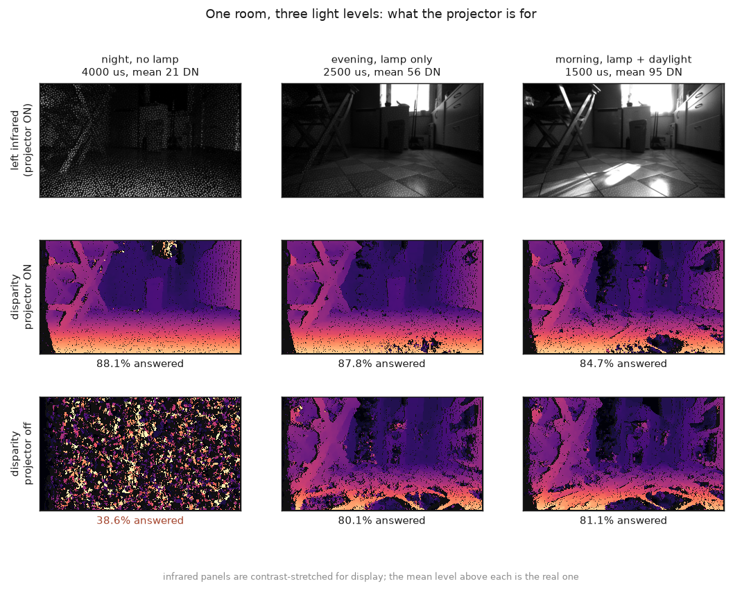
Read the night, no lamp column first, on its projector off row. With no lamp and no projector, the image is sensor noise and nothing else: 0.12 DN of median local contrast, and a disparity map that is speckle at 38.6% coverage. Switch the projector on in the same darkness and the same code answers 88.1%.

The middle row is the point of the whole figure. With the projector on, the matcher barely notices the light level at all — 88.1%, 87.8%, 84.7% across a 4.5× range of scene brightness. Without it, coverage is whatever the room happens to provide: 38.6%, 80.1%, 81.1%. What the projector is worth is exactly what the room does not already supply — 49.5 points at night, 7.7 in the evening, 3.6 in the morning.

The trend in the middle row runs the wrong way: more ambient light makes the projector-lit result slightly worse, 88.1% down to 84.7%. Brighter rooms force a shorter exposure and still clip more of the frame — 0%, 3.4%, 8.6% of pixels at 255 — and a saturated pixel carries no texture at all. The brightest column combines a lamp with morning daylight through a window, the condition a vehicle meets outdoors, and yields the lowest coverage of the three for this matcher.

Exposure is set per condition — 4000, 2500 and 1500 µs — each being the value that holds 3–5 DN of local contrast in that room. One fixed exposure across a 4.5× range of brightness would have measured the exposure rather than the projector.

Those dots also make the Census descriptors 3.3× degenerate on this camera: 338 distinct codes for 1115 keypoints, so many pixels are indistinguishable from one another. That is exactly the ambiguity a one-to-one constraint is for, and exactly where a winner-take-all matcher assigns the same right pixel to several left ones.

1. The split: regular work on the GPU, irregular work on the CPU

The two halves of the matcher differ in kind:

• The cost side is regular. Census, the graded cost, the recursive filter and the top-2 selection touch every (pixel, disparity) pair in a pattern known at compile time. No data-dependent branching, no irregular memory.
• The solve side is irregular. MASDA’s messages and decode walk the claimant lists for each right pixel and apply a greedy one-to-one assignment in score order. It is also small: with two candidates per pixel the whole row problem fits in 28 KB of cache, and four ARM cores handle a full frame in ~11 ms.

Making the solve a GPU kernel would be work spent making the architecture uniform, not work spent making the system faster. So the interface is two scored disparity candidates per pixel — 8 MB per frame instead of the 52 MB int16 cost volume. The GPU reduces; the CPU decides.

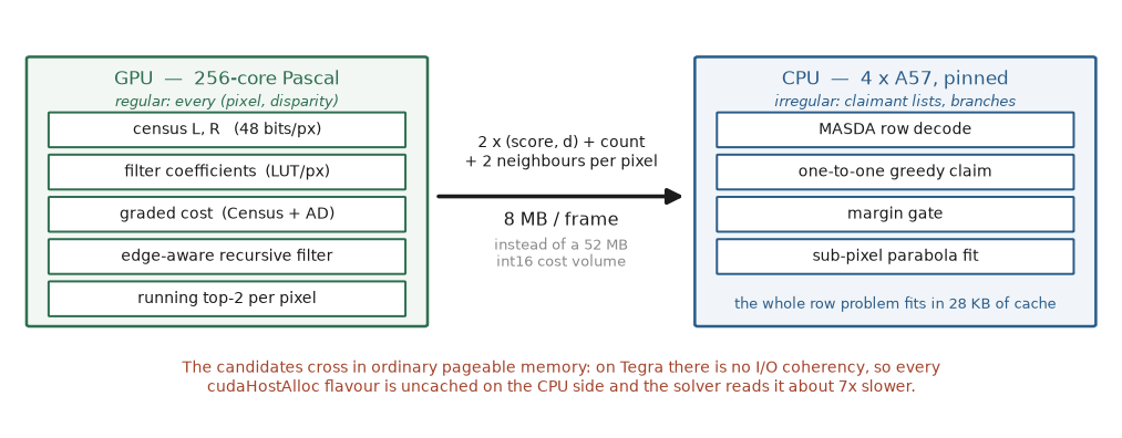
One trap specific to Tegra sits on that arrow. It cost 300 ms twice before I believed it: the TX2 has no I/O coherency. Every kind of cudaHostAlloc memory is therefore uncached on the CPU side — including the kind usually described as “cached pinned”. A solver that reads candidates from such memory runs about seven times slower than from ordinary pageable memory. The candidates travel through a staged cudaMemcpy into a plain std::vector, and the pipeline is where that copy hides.

2. Dataflow: five kernels, two of which are fusions

Per frame, in stream order, with measured kernel minima at 848×480, \(D=64\):

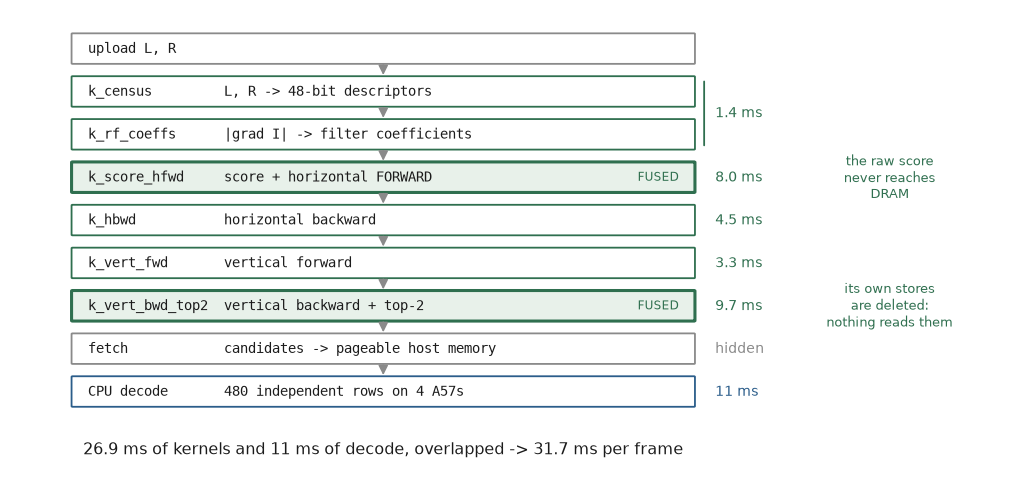
The two fusions are where most of the speed lives, and they follow one principle:

A pass that stores exactly what the next pass reads is a fusion candidate. A store that nothing reads afterwards is a bug costing you time.

The first port scored the volume (52 MB written), read it back to filter (52 in, 52 out), wrote it filtered, then read it again for the top-2. The shipping version computes the score inside the first filter pass and consumes the volume inside the last one. The scored-but-unfiltered volume never makes a round trip and the fully-filtered volume is never materialised at all. What remains in DRAM is the minimum the data dependencies allow — the recurrences genuinely need their intermediate planes.

The sub-pixel fit costs almost nothing on the GPU. Part 2 describes the fit and what it is worth: 41.5% → 24.5% bad-1.0. On the CPU it costs 1.30×, because the two neighbouring costs have to be retained while streaming planes. On the GPU they are already in registers. At the moment the winner is known, the top-2 reduction has the whole disparity range of a pixel live across the warp. Publishing the winner then takes one broadcast, and fetching its neighbours takes two shuffles.

Measured cost: 1.10×. Sending those neighbours to the host in Q14 rather than float halves the extra transfer.

3. The pipeline, and where detection hides

Single-frame latency is ~50 ms. Throughput is 31.7 ms because the GPU computes frame \(t{+}1\) while the CPU works on frame \(t\):

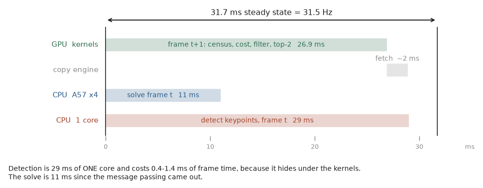
Three details make the overlap real rather than hopeful.

The fetch runs on its own thread. cudaMemcpy serialises with the stream, so the fetcher blocks until frame \(t{+}1\)’s kernels finish and then copies — while the decode of frame \(t\) is still on the A57s. Before this, the copy sat serially in the loop.

The decode threads pin themselves to the A57 cluster. The TX2 has four A57s and two Denver cores. Left unpinned, the threads get moved between the two clusters by the scheduler, and the decode varies between 30 and 45 ms from run to run. Pinned, it sits within half a millisecond of its minimum. The Denvers are left to the CUDA driver and the fetcher. (The same change measured 40% worse on the CPU-only matcher, which needs the Denvers for throughput. An optimisation is a measurement attached to a machine.)

Keypoint detection is a third thread, and it costs nothing. The system needs a sparse feature set as well as a dense map — for tracking and odometry — and detection is 29 ms of one core. Run inside the pipelined loop beside the decode, it costs 0.4–1.4 ms of frame time, because it hides under the 26.9 ms of kernels. 97.3% of detected keypoints then carry a disparity read straight out of the dense map.

That last point is a result, not plumbing. Sampling the dense map at the keypoints beats running the sparse matcher on the same keypoints on every axis: 0.853 precision against 0.706, with 57% more correct matches, and no matcher to run. The sparse matcher’s recall is bounded by whether the right image’s detector also fired within a pixel of the true correspondence, which is a 44–51% repeatability ceiling. A dense map has no such requirement. One producer, two products.

None of this can be said unless detection is measured inside the pipelined loop. Measured outside it, the detection step appeared to cost nothing, and the frame rate looked unchanged for the wrong reason.

4. Why the two machines want opposite layouts

Part 1 and Part 2 kept running into the same question: is the cost volume disparity-major or disparity-minor? The CPU answered three times — disparity-major, because the aggregation filter wants whole constant-disparity planes, and the transpose to the other layout was the dominant memory cost of the early implementation.

The GPU wants the opposite, and the reason is precise:

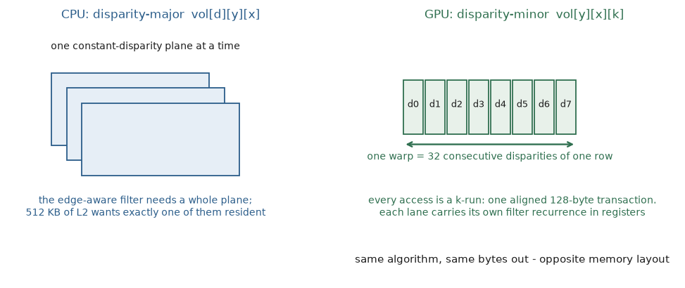
The volume is stored vol[y][x][k] — \(k\) innermost, padded to 64-aligned runs — and a warp is 32 consecutive disparities of one image row:

• The right-census reads for 32 consecutive \(d\) at one \(x\) are 32 consecutive addresses: one coalesced 256-byte window that slides one element per step and lives in L1. The left descriptor and the filter coefficient are the same address for all 32 lanes — a hardware broadcast.
• Every volume access anywhere in the pipeline is a \(k\)-run: an aligned 64- or 128-byte transaction. Nothing strides.
• Each lane carries its own filter recurrence in registers. No lane waits on another, and the filter needs no shuffles at all.

The same assignment appears in ReS2tAC for SGM, on NEON as well as CUDA, and this is the third time this project has re-derived their design point from a different direction. Neither layout was wrong; each machine’s memory system picks its own. A cache hierarchy with 512 KB of shared L2 wants one plane at a time, resident. A latency-hiding machine with 32-wide transactions wants the innermost index to be the one the warp spans. Trying to make one implementation serve both was the actual mistake.

4.1 What one lane actually does

The whole design fits in one kernel. A block covers 64 disparities of one image row, and a thread owns a single disparity. That thread walks the row from left to right, computing the cost and running the horizontal filter as it goes:

// grid: (H rows, D/64 disparity blocks).  blockDim.x = 64 -> two warps.
__global__ void score_and_forward_filter(
    const uint64_t* cl, const uint64_t* cr,   // census, left and right
    const uint8_t*  L,  const uint8_t*  R,    // raw grey, for the AD term
    const uint16_t* ax,                       // filter coefficient, per pixel
    int16_t* vol, int W, int D, int Dpad, int dmin, int32_t wq)
{
  const int lane = threadIdx.x & 31;
  const int y    = blockIdx.x;                            // one row per block
  const int k    = blockIdx.y * 64 + (threadIdx.x >> 5) * 32 + lane;
  const int d    = dmin + k;                              // THIS lane's disparity

  const uint64_t* clr = cl + (size_t)y * W;
  const uint64_t* crr = cr + (size_t)y * W;
  int32_t F = 0;                                          // this lane's recurrence

  for (int x = 0; x < W; ++x) {
    int32_t v = 0;
    if (k < D && x >= 3 + d && x < W - 3) {
      const int32_t c = tbl[__popcll(clr[x] ^ crr[x - d])];      // Census, 0..48
      const int32_t a = adt[abs(int(L[y*W + x]) - int(R[y*W + x - d]))];
      v = (c * (1024 - wq) + a * wq) >> 10;                      // graded cost, Q14
    }
    F = (x == 0) ? v                                             // the filter, fused
                 : v + ((ax[y*W + x] * (F - v) + (1 << 14)) >> 15);
    if (k < D) vol[((size_t)y * W + x) * Dpad + k] = (int16_t)F;
  }
}

Two lines carry the entire argument for this layout.

F is a register. The edge-aware filter is the awkward, sequential part of the algorithm, and here it needs no shared memory, no shuffles and no synchronisation. 32 independent recurrences run side by side, because they are 32 different disparities of the same row. And the score is never stored before it is filtered. v is consumed by the recurrence in the same instruction stream that produced it, which is the fusion that deletes a 52 MB round trip through DRAM.

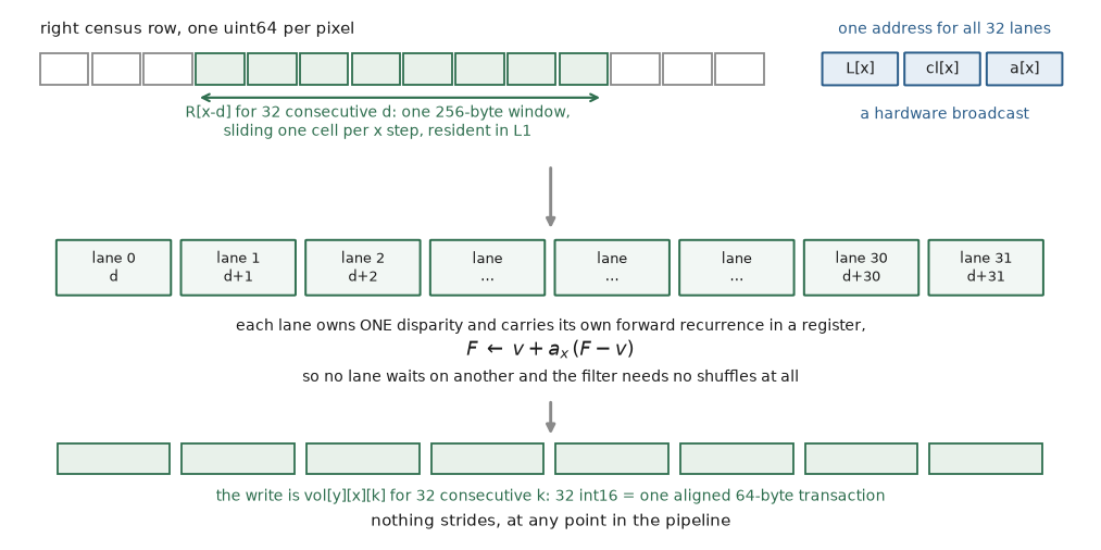
The addresses are worth doing once, because “coalesced” is a claim and this is the arithmetic behind it. With \(D_{\text{pad}} = 64\), a pixel’s disparity run is \(64 \times 2 = 128\) bytes and starts on a 128-byte boundary:

• the write, vol[(y·W + x)·64 + k] for 32 consecutive \(k\): 32 int16 at consecutive addresses — one aligned 64-byte transaction, for the whole warp;
• the right census, crr[x - d] for \(d = d_0 \dots d_0+31\): 32 consecutive uint64 — a 256-byte window that slides by exactly one element when \(x\) advances, so it stays in L1;
• everything else — clr[x], L[x], ax[x] — is the same address in all 32 lanes, which the hardware serves as a broadcast rather than 32 loads.

4.2 How the top-2 comes out of the warp

The solver wants two candidates per pixel, and after the vertical backward pass the 64 filtered costs of a pixel are spread across the warp, two per lane. Getting the best two out is a reduction across lanes, done with __shfl_down_sync in five rounds:

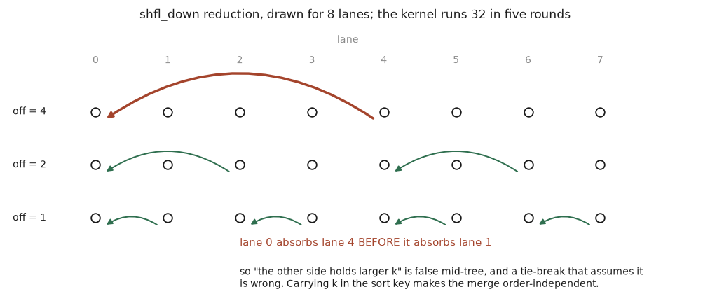
The subtlety is the tie. The CPU walks \(k\) ascending and needs a strictly greater score to displace the incumbent, so among equal scores the smallest \(k\) wins. The warp does not walk anything in order. Lane 0 absorbs lane 16 before it absorbs lane 1. So a rule like “the other side holds the larger disparities” is simply false in the middle of the tree.

The fix is to stop breaking ties at all, by putting \(k\) into the sort key:

The score occupies the high bits and \(255-k\) the low eight, so a plain integer > is the ordering “score descending, then \(k\) ascending”. Two candidates that tie at \(s = 1000\) give \(\text{key}(1000, 5) = 8{,}644{,}858\) against \(\text{key}(1000, 17) = 8{,}644{,}846\): the smaller disparity wins by construction, whichever lane it arrives from. The merge becomes order-independent, and it costs two shuffles per round instead of a comparison chain. Eight bits are enough for \(k\) because \(D\) reaches 220 at its widest.

article/top2sim.py reproduces the tree on the host in twenty lines and counts the disagreements against the CPU’s scan:

Ties are the only case the two keys can disagree on, so the error rate is a direct function of how many of them there are. A real Q14 cost volume has few, which is why this bug arrived as ten wrong pixels in 407,040. That is nowhere near visible to an accuracy benchmark. It was caught only because the GPU is held byte-identical to the CPU.

5. What the board delivers

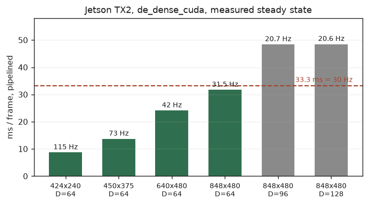
Measured steady state, pipelined over 30 frames, best of three at locked clocks:

Disparity range costs in steps of 64, because the \(k\)-runs pad to a multiple of

1. The step is the whole story: \(D=32\) measures 25.5 ms in the cost stage and \(D=64\) measures 25.6, while \(D=65\) measures 41.8 and \(D=128\) measures 42.4. So \(D=128\) costs nothing if you are already computing \(D=96\), and asking for fewer than 64 disparities saves nothing at all — it computes the same block and discards part of it. \(D=64\) is therefore the only sensible setting below the step, and the matcher runs there. 848×480 at \(D=64\) closes 30 Hz at 95% of the frame budget. No other configuration does. On a vehicle the board will get hot and slow itself down, which reduces that margin. When it does, the pipeline drops to 15 Hz instead of failing.

That step has a consequence outside the timing table. The live pipeline had its minimum range set to 0.4 m, which is \(D=53\). That sits inside the same block of 64, so the missing eleven disparities were already computed and thrown away. Everything nearer than 0.4 m came back as a confident wrong answer rather than as a gap.

Fixing it cost nothing measurable: 32.0 ms at \(D=53\) against 31.7 at \(D=64\).

The 848×480 rows are measured on a recorded IR pair from the camera. The smaller resolutions are Middlebury scenes at their native sizes.

6. What did not work

A warp-serial scan of the recurrence: 55.7 ms, worse than what it replaced. The recursive filter is the hardest part to port. It is a recurrence: every step depends on the one before it, in integer arithmetic, with truncation. So the classic block-parallel formulation (Nehab et al.), which reassociates the filter algebraically, cannot reproduce it bit-exactly. My first alternative kept bit-exactness by loading coalesced rows and stepping through the 32 lanes one at a time via warp shuffles. It was coalesced and bit-exact, but 31 of the 32 lanes sat idle at every serial step. The limit was instruction throughput, not memory bandwidth. The \(k\)-minor layout removed the question entirely: a lane per disparity rather than per position means every lane runs its own recurrence.

An ordered tie-break in the top-2 reduction: ten wrong pixels in 407,040. The mechanism and the fix are in how the top-2 comes out of the warp. The part that belongs here is that assuming an order across a shuffle tree is a mistake worth naming.

Every one of the ten differing pixels was an exact score tie. A five-million-run host simulation of the precise shuffle tree reproduced it. The fix packs (value, \(k\)) into a single integer whose plain comparison is (value descending, \(k\) ascending), and is therefore order-independent. That simulation now runs in make test.

A compile-time run length: six of eight scenes silently wrong. The \(k\)-runs were padded to a hard-coded 64, and six of the eight ground-truth scenes need \(D=80\). Their upper disparities were never scored, and the top-2 read into the neighbouring pixel’s run. The two scenes that passed — Teddy and Cones — are exactly the two everything gets tuned on, at \(D=60\).

Mapping the GPU’s speed-ups back to the CPU: mostly no. Fusing the top-2 insert into the filter’s last pass is the GPU’s single biggest speed-up. On the CPU it changes nothing — the plane sits in L2 between passes, so the store the fusion deletes cost almost nothing and the re-read was nearly a cache hit. A first version was 18% worse, because putting a branchy insert inside the recurrence loop killed the compiler’s autovectorisation.

7. Bit-identity as the referee

The whole port was built under one rule: every intermediate keeps the CPU’s exact integer arithmetic, so cmp on the final disparity map is the test. The census bit order, the Q14 tables with C++ truncating division, the filter’s int32-carry/int16-store pattern, the ascending-\(k\) strictly-greater top-2 — all replicated.

This costs something. The Nehab-style filter was off the table, and so is any reassociation. It has justified that cost three times. The tie bug and the padding bug are both invisible to an accuracy benchmark at the scale they occur, and a race in the pipelined mode would be invisible too. The pipelined path writes the last frame’s output, so a broken overlap breaks the identity check instead of passing quietly.

It also means the accuracy story needs no new evidence. The GPU produces the same bytes, so Part 2’s measurements are the GPU’s measurements. That includes the ones that went against expectation: the sub-pixel fit reducing bad-1.0 by 17 points, and the message passing not being worth its cost in the dense path.

7.1 The whole frame in one table

Every stage above, in stream order, with what it consumes and produces. Kernel times are measured minima at 848×480 and \(D=64\); the two fused stages are marked.

Three conditions make those numbers hold, and each is measured above:

• The decode and the detection run on frame \(t\) while the kernels run on frame \(t{+}1\). Without that overlap the frame costs 26.9 + 11 ms instead of 31.7.
• The decode threads pin themselves to the A57 cluster. Unpinned, the decode varies between 30 and 45 ms.
• The candidates are fetched into pageable host memory. Pinned memory is uncached on this SoC, and a solver reading from it runs about seven times slower.

8. Where this leaves the project

The matcher runs at the camera’s full resolution, faster than the camera delivers frames, on a computer that costs less than the camera. It gives the rest of the system two products from one pass: a dense disparity map, and a sparse feature set whose disparities are better than the ones a dedicated sparse matcher produced.

What is genuinely unfinished:

• Coverage, and accuracy at equal coverage. At the shipping gate this matcher answers 80% of pixels and SGM answers 90%.

  Compare them at the same coverage and SGM is ahead there too. Part 2’s precision–coverage curve plots error rate against coverage, so a lower curve is a better one. SGM sits about two points of error below this matcher, across the range where the two overlap. That gap was three points before the equiangular estimator.

  No parameter setting closes it. A parameter moves the operating point along the curve; closing the gap means moving the curve itself. Part 2 tried four structural changes for that, and none of them worked.

• The descriptor, which is the largest single item in the error budget. 10.8% of far-field pixels have no candidate within half a pixel anywhere in the top eight, so no solver on this cost volume can reach them. Part 2’s parameter table measures that a bigger Census descriptor only trades along the precision–coverage curve, which means the gap is in the similarity function rather than in its resolution. This is the one place where the learned costs at the top of the Middlebury table beat this design. It is deliberately out of scope: the GPU is already at 95% of the frame budget, so nothing neural fits behind it.
• The selector. 13.1% of far-field pixels have the truth sitting in the top-2 with the top-1 taken. Neither winner-take-all nor MASDA’s message passing collects it — they measure within a point of each other — so this is a real mandate with no mechanism currently addressing it. With two candidates it is a binary choice per pixel, and the one thing that has never been tried on it is a term that couples neighbouring pixels across rows. MASDA’s uniqueness runs along a row only.
• Occlusion. Pixels within 8 px of a depth discontinuity carry 28.6% of all error, and neither a sharper edge-aware filter nor a wider candidate set moves them. What is left is half-occlusion: part of the support window has no counterpart in the other image at all. That is a different problem from the one the aggregation solves.
• The temporal direction, which is where MASDA’s own claim is still open. Part 2’s ablation says the message passing is not worth its cost when it decides between two candidates on a rectified row. Frame-to-frame association is the opposite situation: the candidate set is large, two-dimensional, and genuinely ambiguous, and there is no dense map of the motion to read instead. That is the experiment the series has been building toward, and it has not been run yet.

References

Full citations with DOIs, and every term this post uses, are in the series glossary.

• Ruf, B., Mohrs, J., Weinmann, M., Hinz, S., & Beyerer, J. (2021). ReS2tAC — UAV-borne real-time SGM stereo optimized for embedded ARM and CUDA devices. Sensors, 21(11), 3938 — disparity-in-the-lanes, and the embedded CUDA baseline this design is measured against.
• Nehab, D., Maximo, A., Lima, R. S., & Hoppe, H. (2011). GPU-efficient recursive filtering and summed-area tables. ACM Transactions on Graphics, 30(6), 176 (SIGGRAPH Asia) — the block-parallel recursive filter, and by its existence the explanation of why a warp-serial scan loses.
• Parts 1 and 2 of this series — the derivation, and the matcher this post makes real-time.