A stereo matcher produces a depth for almost every pixel. Roughly one in ten of them is wrong, and the matcher does not say which. Everything downstream then has to treat a measurement it can rely on and one it invented as the same kind of thing: a temporal filter votes on them equally, an occupancy grid carves free space out of both, and a planner steers around a surface that is not there.
This post is about giving each point a number that says how much it is worth, using only what the matcher already computed. No network, no second pass over the image, and in the end one logarithm and one division per pixel.
Three results are worth reading even if you never touch this code. A confidence measure and a probability are different things, and the difference is not presentational. A textbook trick can be exactly right and buy nothing, if the pipeline already does it somewhere you did not look. And the model that fits your benchmark best can be the one you must not deploy, because it fits best precisely where your benchmark has no examples.
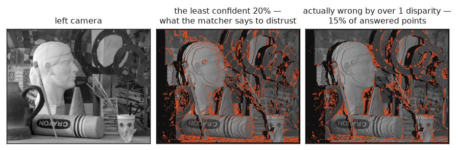
Middlebury’s Art scene. The centre panel is the fifth of points this post’s measure
distrusts; the right panel is the points that are actually wrong by more than one
disparity. Neither picture was drawn by hand — both come out of the shipping matcher.
1. Where the information already is
A stereo matcher compares each pixel of the left image against a row of candidates in the right image and keeps the best, which fixes that pixel’s disparity and so its depth. The version I am measuring keeps the best two, because its solver needs a runner-up, and those two numbers are enough to distinguish situations that the disparity map alone flattens together:
| best score | runner-up | what it means | |
|---|---|---|---|
| pixel A | 0.90 | 0.30 | the winner is far ahead. Probably right. |
| pixel B | 0.52 | 0.51 | a coin flip that happened to land. Probably wrong. |
Both come out of the matcher as a disparity, with nothing to separate them. The information exists; it is simply discarded.
There are two obvious ways to turn a pair of scores into one number: subtract them, or divide them. Both are named in the literature. Hu and Mordohai’s survey of confidence measures calls the difference maximum margin, naive and the ratio peak ratio, naive, and they are among the oldest and simplest measures in the field. My matcher already shipped the difference, as a hard gate. Nobody had measured which of the two is better.
2. How you tell whether a confidence is any good
Throw away the least confident points and see whether the error rate falls.
Sort every answered point by confidence, keep the top fraction \(q\), and record the error rate among what is kept. That is the sparsification curve \(e(q)\), and the area under it,
\[\mathrm{AUC} \;=\; \frac{1}{N}\sum_{q} e(q), \qquad q = 1.00,\, 0.99,\, \dots,\, 0.01\]is one number for the whole curve, lower being better. It has been the standard metric in this corner of stereo since Hu and Mordohai fixed it, and two reference curves make it readable:
- an oracle, which sorts by the true error and therefore discards every wrong point first. Its area is the floor nothing can beat.
- a random confidence, whose curve is flat at the overall error rate. Its area is the no-skill ceiling. A measure that does not beat it is noise.
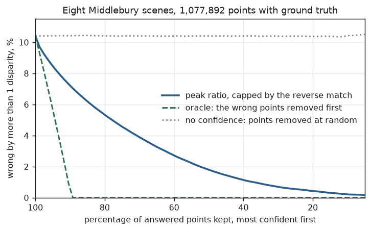
On eight Middlebury scenes — 1,077,892 points with ground truth, matched with the gate switched off so nothing is scored on a population it has already filtered — the population is 10.4% wrong. The measure below closes about three quarters of the distance between chance and the oracle, and the practical reading is the curve itself: keep the best 60% of points and three quarters of the errors are gone; keep the best 40% and it is nine in ten.
| measure | AUC | error at 60% kept |
|---|---|---|
| oracle | 0.0062 | 0.0% |
| peak ratio | 0.0294 | 2.7% |
| the margin, which was already shipping | 0.0344 | 3.5% |
| random | 0.1041 | 10.4% |
The ratio beats the difference, on the same two numbers, for one divide instead of one subtract.
3. The textbook trick that bought nothing, and why
The most useful single finding in the modern literature on this is Poggi, Tosi and Mattoccia’s re-evaluation of 52 confidence measures, and it is unambiguous: local aggregation is what separates a good hand-crafted measure from a poor one. The peak ratio pooled over a small window — APKR — ranks in the top handful of hand-crafted measures, while the per-pixel version does not.
I implemented it. It did nothing at all: AUC 0.0294 either way, and worse with a bigger window.
The reason turned out to be worth more than the feature would have been. My matcher runs an edge-aware recursive filter over the cost volume before it picks the top two, with a spatial reach of about six pixels. The neighbourhood the textbook wants to pool over is already inside the neighbourhood the filter covered. Pooling again adds no evidence, and past the filter’s reach it only smears confidence across depth edges.
That is a hypothesis, so it needs a test that can fail. Turn my own filter down and the published effect should reappear:
| aggregation strength \(\sigma_s\) | 1 | 2 | 8 (shipping) | 20 |
|---|---|---|---|---|
| peak ratio | 0.0513 | 0.0349 | 0.0294 | 0.0339 |
| pooled over 5×5 | 0.0418 | 0.0316 | 0.0294 | 0.0340 |
| what pooling bought | 0.0095 | 0.0033 | 0.0000 | −0.0001 |
It does. The literature is right and the feature is redundant here, which are not the same statement. A measure that is worth a window on a raw cost volume is worth nothing on an aggregated one — and the only way to know which pipeline you have is to try it.
4. The blind spot no cost curve can see
Everything above reads the shape of one pixel’s cost curve: how far ahead the winner is. That family shares a structural weakness.
Consider a pixel whose true match lies outside the searched range, or off the edge of the sensor entirely. It has no correct candidate to lose to. The best of the wrong candidates wins by a wide margin, the ratio is excellent, and the measure reports high confidence in an answer that is not merely inaccurate but meaningless. On my camera this appears as a second, phantom floor sloping away beneath the real one — confident, coherent, and completely invented.
The classical cure is left-right consistency. Match left to right, then ask the right pixel that was claimed which left pixel it would have chosen. If the two disagree, one of them is wrong.
The usual objection is cost: it looks like a second matching pass. It is not, because the scores already exist. The cost volume holds the score of left pixel \(x\) against right pixel \(x-d\) for every pair. The forward match reduces those over \(d\) for each \(x\); the reverse match reduces the same numbers over \(x\) for each \(x-d\). It is a second running maximum in the loop that already holds the score:
const float v = slice[i];              // i indexes the LEFT pixel
if (trs) {                             // before the reject below — see the note
  const size_t j = i - size_t(d);      // the RIGHT pixel this same score belongs to
  if (v > trs[j]) { trs[j] = v; trd[j] = kk; }
}
if (v <= ts1[i]) continue;             // the forward path's early-out
The ordering is the whole subtlety. That early-out discards almost every score, because it cannot beat this left pixel’s runner-up. The same score may still be the best any right pixel has seen. Build the reverse match after the reject and you build it from the few per cent that happened to survive — silently, and it still looks like an answer.
Is this not what a one-to-one constraint already does?
Partly, and the overlap is worth being precise about, because it is easy to assume the work is redundant.
A matcher that enforces uniqueness — at most one left pixel per right pixel — resolves collisions between winners: two left pixels claim the same right pixel, the stronger claim takes it, the loser gets no answer. The reverse match asks a wider question, of every candidate rather than only the winners:
Left 10’s best is right 9, at 0.82. Nothing else is close, so it looks confident. Left 12’s best is right 7 — but its second choice is right 9, at 0.91.
Left 12 never claims right 9, so uniqueness sees no collision and lets left 10 through. Right 9’s true best partner is left 12. The reverse match sees that; uniqueness cannot.
Measured on my matcher, which enforces uniqueness: 3.0% of the points it answers fail the reverse match. All of those passed uniqueness. Everything below is measured on top of it, never instead of it.
5. The result that changed how the cue is used
Having built it, the obvious step is to fit it: two features, one logistic regression, let the data choose the weights. That produced a model whose numbers looked fine and which would have been a mistake to ship.
Splitting the data by the reverse match and by how strong the ratio is:
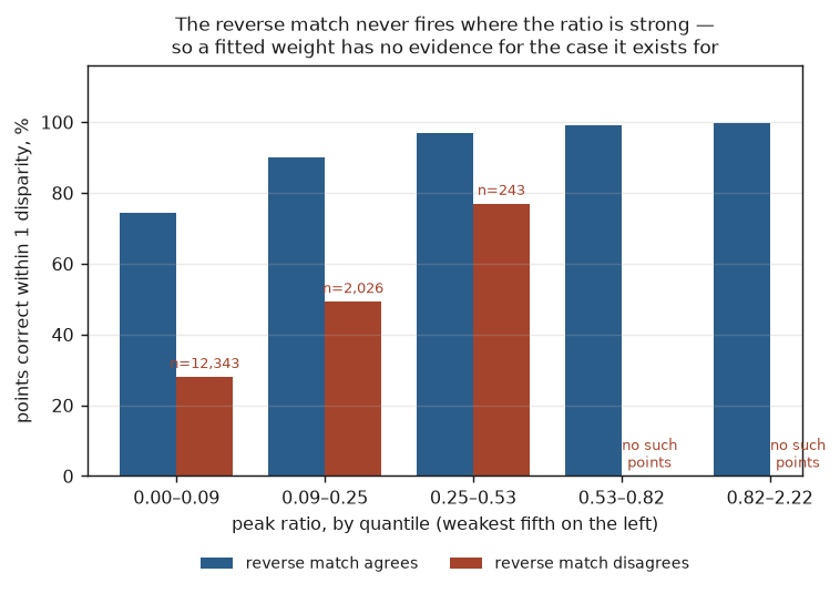
Two things at once. Where the check fires it separates hard — 74.5% correct against 28.0% inside the same ratio band. And it essentially never fires where the ratio is strong. In the two strongest quintiles, out of 269,000 points, there are none at all.
So a fitted weight has no evidence for the one case the cue exists for. Handed a point with a confident ratio that the reverse match rejects, the fitted model extrapolates into an empty region and returns 0.998. That combination is exactly the phantom floor: a match with no true competitor scores a confident ratio, and the reverse match is the only thing that objects.
The fitted offset calibrates better on the benchmark — 0.0088 against 0.0133 — and it is unusable for precisely the reason it looks good. Middlebury contains no examples of the failure, so the fit is free to say anything there, and what it says is wrong.
What ships instead is a hard cap. Where the reverse match disagrees by more than a disparity, the confidence is capped at 0.35 — the measured correctness of that population, 31.8% against 89.6% for everything else. Both variants reach the same benchmark score, 0.0288. Only one of them refuses to extrapolate where it has no evidence.
The whole model is then two lines:
const float alt = (s2 > -1e29f) ? std::max(s2, lambda) : lambda;
const float x   = std::log(std::max((1.f - alt) / std::max(1.f - s1, 1e-6f), 1e-6f));
const float p   = 1.f / (1.f + std::exp(-(0.692684f + 7.936751f * x)));
return (lrc > 1.f) ? std::min(p, 0.35f) : p;
Evaluated at the eight-scene mean, \(s_1 = 0.682\) and \(\mathrm{alt} = 0.537\): \(1 - s_1 = 0.318\), \(x = \log(0.463/0.318) = 0.3757\), so the logit is \(0.692684 + 7.936751 \times 0.3757 = 3.674\) and \(P = 0.975\).
A single feature, on purpose
Richer versions were tried and rejected, and the reason is a second case where a linear model cannot say what needs saying.
A region with no texture has a constant descriptor, so every disparity matches it perfectly. Then \(s_1 = s_2\): the margin is zero, the ratio is one, and both cues correctly report no information. But a model that also reads the winning score sees a perfect score and returns 0.94. It cannot express “a high score only counts when the margin is not zero”, because that is a product and it is a sum — and it was never shown such a pixel, because Middlebury is textured almost everywhere.
I found this by padding a test frame with black. The padding scored higher than the real image beside it. The single-feature model returns 0.667 there, below anything a real match reaches, and a unit test now holds it to that.
6. Is it a probability?
Ranking and calibration are different properties, and a measure can have one without the other. Fitted by leave-one-scene-out regression — every prediction made by a model that never saw its scene — the answer on the benchmark is yes. Binned by what it promised, over held-out points:
| promised | delivered |
|---|---|
| 0.15 | 0.11 |
| 0.45 | 0.42 |
| 0.76 | 0.77 |
| 0.86 | 0.86 |
| 0.97 | 0.97 |
Mean gap 0.005. A predicted 0.8 means 80%.
And that pooled number hides a factor of fifteen. Per held-out scene the gap runs from 0.013 to 0.080, and the direction is the problem: on the hardest scene it promises 0.879 and delivers 0.798. It regresses towards the difficulty of the mix it was trained on, so on anything harder than that mix it is over-confident — which is the dangerous direction. A pooled calibration figure should never be quoted without the per-scene column beside it.
7. What it does not know, on a real camera
Middlebury is a benchmark. The camera this runs on is an infrared stereo pair with a dot projector, on a Jetson TX2. Whether any of this transfers to it is a separate question, and it has to be measured there.
Against a flat wall — the cheapest ground truth there is, since scatter about a fitted plane is the matcher’s noise — it does. 6.2% of points sit more than 20 mm off the wall, falling to 1.3% keeping the best 60%, and the measure closes 74% of the distance to an oracle against 76% on Middlebury. The ordering carries over.
The absolute number does not: it promises 0.86 on that wall and delivers 0.94. Pessimistic here, optimistic on the hardest benchmark scene, and fitted on neither.
Then six captures of one kitchen at three light levels, with the projector on and off:
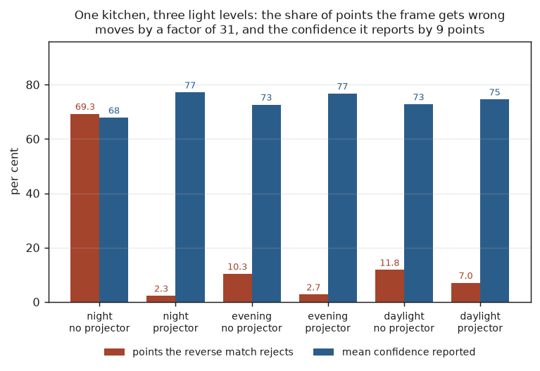
The share of points the frame gets wrong moves by a factor of thirty-one. The mean confidence it reports moves by nine points. The measure orders points well inside a frame and knows almost nothing about how good the frame is.
That has a direct practical consequence, and it is the one I would most like a reader to take away. A fixed threshold — “keep everything above 0.85” — keeps 6% of points in one condition and 18% in another. It throws away most of a good cloud and retains a sixth of a hopeless one. Threshold on the fraction instead: “keep the best 40% of this frame” behaves identically at midnight and at noon, because it is a quantile of a distribution rather than a point on an uncalibrated scale.
The exception is the first pair of bars: in a dark room with the projector off, the frame carries 0.12 DN of local contrast and 38.6% of pixels get any answer at all. No threshold and no quantile helps there. That is a frame to refuse, and refusing it needs a feature describing the whole frame rather than each pixel — which is the next thing to measure, and is not measured yet.
8. What this cost
Nothing that shows up in a profile. The two scores were already computed by the matcher’s own reduction. The reverse match reuses buckets the solver already builds and then discards — its message-passing update needs exactly that structure — so it is two loops over scratch memory that was already dead. The model is a logarithm, a divide and an exponential. Per point, the live pipeline sends one extra byte.
The exact reverse match, over all 64 disparities rather than the two candidates that survived, would be worth roughly twice as much again. It is the one piece here that is genuinely expensive: on a k-minor cost volume the reverse reduction runs along a diagonal, which is uncoalesced by construction, and doing it on the GPU means about 26 million atomic maximums per frame on a device already at 26 ms of kernels in a 28.9 ms budget. That is a trade to make on evidence, not on principle.
9. What I would tell someone starting this
- Check what your pipeline already does before adding a published feature. Local aggregation is the single most valuable idea in the confidence literature and it was worth exactly zero here, because the cost volume was already filtered. The measurement that establishes this — turning my own filter down until the published effect reappears — took ten minutes and saved a kernel.
- A cue that fires only in one corner of your data cannot be fitted as a weight. Check where a feature is active before letting a regression decide what it means. If it never co-occurs with the case you care about, the fit is unconstrained exactly there.
- Rank first, calibrate second, and never quote a pooled calibration alone. Sparsification measures ordering. It says nothing about whether 0.8 means 80%, and pooling across scenes can hide a factor of fifteen by letting optimism on hard scenes cancel pessimism on easy ones.
- Test the degenerate input. A blank wall, a black frame, a saturated one. My worst bug was found by padding a test image with zeros, and no benchmark number moved when it was present.
The matcher this is built on is described in an earlier series — the formulation, the dense C++ implementation and the real-time GPU port — but nothing above depends on it. Any stereo matcher that keeps two candidates per pixel has these numbers already, and is throwing them away.
References
- X. Hu and P. Mordohai, A Quantitative Evaluation of Confidence Measures for Stereo Vision, IEEE Transactions on Pattern Analysis and Machine Intelligence 34(11), 2012 — the founding survey, the taxonomy the names above come from, and the sparsification metric.
- M. Poggi, F. Tosi and S. Mattoccia, On the Confidence of Stereo Matching in a Deep-Learning Era: A Quantitative Evaluation, IEEE Transactions on Pattern Analysis and Machine Intelligence, 2021 — 52 measures over five datasets, and the finding that local aggregation is what makes a hand-crafted measure good.
- D. Scharstein and R. Szeliski, Middlebury Stereo Datasets — the ground truth every number on the benchmark side of this post is scored against.