This is the dense stereo matcher: a C++14 implementation of MASDA — max-sum loopy belief propagation for data association — applied to every pixel of an 848×480 infrared pair, on a Jetson TX2. Part 1 derives the message equations and measures the one-to-one constraint on sparse keypoints. This post is the algorithm at full frame rate: the representation it needs, the parameters that matter, the ones that turn out to do nothing, and a set of experiments that ended with a result I did not expect about the algorithm the series is named after.
Every term is defined in the series glossary, with links to the original papers. Terms link there on first use.
The matcher, in one paragraph. Each left pixel is a measurement; its candidate “objects” are the right pixels along the same rectified row within the disparity range. A Census descriptor plus a truncated absolute difference scores every (pixel, disparity) pair; an edge-aware recursive filter aggregates those scores; the two best-scoring disparities per pixel are kept and everything else is discarded. MASDA then solves each row as an assignment problem via its messages with clutter and misdetection, and emits a disparity plus a margin — the gap between the best and second-best candidate — which is the confidence a downstream gate consumes.
Where it stands, measured on the fifteen Middlebury v3 training scenes under the benchmark’s own scoring rules:
| bad-1.0 | coverage | |
|---|---|---|
| dense MASDA | 24.5% | 79.6% |
| Middlebury’s SGM reference | 29.1% | 90.2% |
Ahead on the error rate over answered pixels, ten points behind on how many pixels it answers. The whole curve is below, which is the only fair way to read a matcher that declines to answer.
1. The cost volume is never built
The textbook pipeline materialises a \(W \times H \times D\) cost volume — at \(D=64\) that is 43 MB per frame at 450×375 and 104 MB at 848×480 in float, or half of each once the scores are Q14 int16 — aggregates it, then reads it back to pick winners. I built that first, then measured what the solver actually consumes.
1.1 The score, one pixel at a time
Before anything is aggregated there has to be a number to aggregate, and it comes from comparing two small patches. The Census transform describes a pixel by how its neighbours compare with it, and nothing else:
\[\mathcal{C}(p) \;=\; \Big(\, \big[I(q_1) < I(p)\big],\; \big[I(q_2) < I(p)\big],\; \dots,\; \big[I(q_{48}) < I(p)\big] \,\Big)\]For a 7×7 window that is 48 neighbours, so 48 bits packed into a uint64. The centre
pixel is not coded — it is the thing everything is compared against. What survives is
the ordering of brightness in the window, not the brightness itself, which is why the
descriptor does not care that the two cameras have different gain or that one side of
the scene is lit more strongly than the other.
Two descriptors are compared by Hamming distance — count the bits that disagree — which is one instruction:
\[h(p, q) \;=\; \operatorname{popcount}\big(\mathcal{C}(p) \oplus \mathcal{C}(q)\big) \;\in\; [0, 48]\]Here it is on one pixel of Teddy, at its true disparity and 5 px away from it:
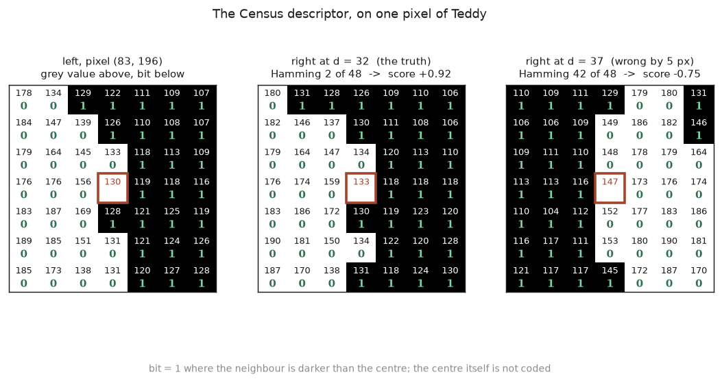
The left patch codes to 0xe1c3c71c3c7c. At the true disparity the right patch differs
in 2 bits of 48; five pixels away it differs in 42, which is closer to inverted
than to equal. That is the whole matching signal, and the figure is also a fair warning
about what happens when a patch has no texture: every neighbour on one side of the
centre, an all-zero code, and no signal at all.
The distance becomes a score on a fixed scale, positive for agreement:
\[s_{\text{census}}(h) \;=\; \frac{24 - h}{24} \qquad\text{so } h=0 \to +1,\; h=24 \to 0,\; h=48 \to -1\]which is \(+0.92\) at the true disparity above and \(-0.75\) at the wrong one. In the code this is a 49-entry lookup table in Q14 — \(s \cdot 2^{14}\) — so the whole cost is integer arithmetic from here on.
One term is blended in beside it. The truncated absolute difference compares the raw grey values, saturating at \(T = 10\) levels:
\[s_{\text{ad}}(v) \;=\; 1 - \frac{2\min(v, T)}{T}, \qquad s \;=\; (1 - \alpha)\, s_{\text{census}} \;+\; \alpha\, s_{\text{ad}}, \quad \alpha = 0.15\]Census carries the structure and is blind to a constant offset; the absolute difference notices an offset but is helpless on flat texture. What the parameters are worth measures what that blend is actually buying, and the answer is not what it was when the term was added.
1.2 What “aggregate” means here
Aggregation is the stage that does most of the work, so it is worth being precise about it.
The problem it solves. One pixel does not carry enough evidence to pick a disparity. A 7×7 Census descriptor compares 48 neighbours, so the score between two pixels is a Hamming distance between 0 and 48 — only 49 possible values. On a surface with little texture, many disparities produce the same score, and the best one is often not the correct one.
The effect is not marginal. On Teddy, taking each pixel’s best unaggregated score lands within 1 px of the truth for 62.0% of pixels; aggregating first takes that to 86.9%. Panel (b) below is one such pixel: the per-pixel score peaks at \(d = 10\) where the truth is 18.25, and after aggregation the peak sits at 18.
What the stage does. For each disparity \(d\), it replaces every score by a weighted average of the scores around it:
\[\tilde{C}(x, y, d) \;=\; \sum_{(u,v)} w\big((x,y),(u,v)\big) \; C(u, v, d)\]Read the indices carefully, because one detail decides the whole design. The sum runs over positions \((u,v)\). The disparity \(d\) is fixed. Aggregation averages a pixel with its spatial neighbours at the same disparity, and never across disparities. That is why the code needs a whole disparity plane — the entire image scored at one fixed \(d\) — in memory at once, and it is the constraint behind two of the negative results later in this post.
The weights are not a fixed window. Averaging across an object boundary is harmful: it pulls a foreground disparity onto the background behind it. So the weight between two neighbouring pixels shrinks when the image brightness changes between them. For a horizontal neighbour pair the coefficient is
\[a \;=\; \exp\!\left(-\frac{\sqrt{2}}{\sigma_s}\left(1 + \frac{\sigma_s}{\sigma_r}\cdot\frac{|\Delta I|}{255}\right)\right) \;=\; \underbrace{e^{-\sqrt{2}/\sigma_s}}_{\text{how far support reaches}}\;\cdot\; \underbrace{e^{-\sqrt{2}\,|\Delta I| / (255\,\sigma_r)}}_{\text{how easily an edge stops it}}\]where \(|\Delta I|\) is the brightness difference between the two pixels, in grey levels. The two knobs are separate: \(\sigma_s\) sets the reach on a flat surface, \(\sigma_r\) sets how large a brightness step has to be before support stops there.
How it is computed. Not with a window. The filter is a first-order recurrence — each pixel mixes its own score with the running value from the previous pixel:
\[F_x \;=\; (1 - a_x)\, C_x \;+\; a_x F_{x-1}\]This runs four times over the plane: left to right, right to left, top to bottom, bottom to top. Each pass costs one multiply and one add per pixel, and that cost does not depend on \(\sigma_s\). A wider support is free. This is why the \(\sigma_s\) sweep later in this post changes accuracy at no cost in time, and why a value that was too large could sit unnoticed.
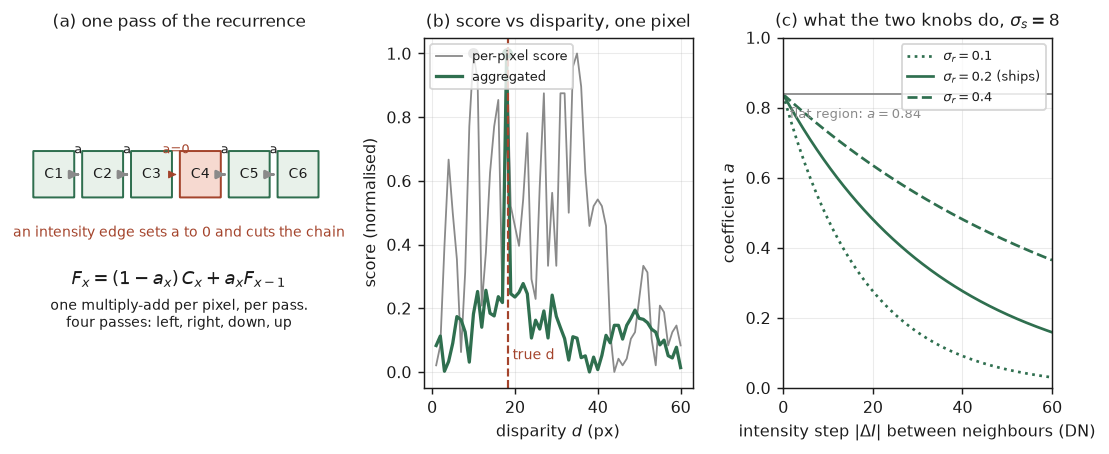
The reach is easy to read off the recurrence. On a flat surface \(a\) is constant, so a pixel \(k\) steps away contributes \(a^k = e^{-\sqrt{2}k/\sigma_s}\). The weight falls to \(1/e\) after \(k = \sigma_s/\sqrt{2}\) pixels. At the shipping \(\sigma_s = 8\) that is \(a = 0.838\) and a reach of 5.7 px, with half weight already at 3.9 px. At a 30-grey-level edge with \(\sigma_r = 0.2\) the coefficient drops to \(a = 0.36\), so support dies about four times faster — which is what “the filter stops at edges” means numerically.
The whole stage is about fifteen lines. This is the shipping filter, written in NumPy instead of C++:
import numpy as np

def coefficients(img, sigma_s=8.0, sigma_r=0.2):
    """One coefficient per neighbour pair. Depends on the image only."""
    k, rs = -np.sqrt(2) / sigma_s, sigma_s / sigma_r
    img = img.astype(np.float32)
    dx = np.abs(np.diff(img, axis=1, prepend=img[:, :1]))   # left neighbour
    dy = np.abs(np.diff(img, axis=0, prepend=img[:1, :]))   # upper neighbour
    return (np.exp(k * (1 + rs * dx / 255)),
            np.exp(k * (1 + rs * dy / 255)))

def aggregate(C, ax, ay):
    """Filter ONE disparity plane in place. Four passes, O(1) per pixel."""
    for x in range(1, C.shape[1]):              # left to right
        C[:, x] += ax[:, x] * (C[:, x - 1] - C[:, x])
    for x in range(C.shape[1] - 2, -1, -1):     # right to left
        C[:, x] += ax[:, x + 1] * (C[:, x + 1] - C[:, x])
    for y in range(1, C.shape[0]):              # top to bottom
        C[y] += ay[y] * (C[y - 1] - C[y])
    for y in range(C.shape[0] - 2, -1, -1):     # bottom to top
        C[y] += ay[y + 1] * (C[y + 1] - C[y])
    return C
Ten pixels of one row, with real numbers — the same row and disparity as the Census example above, before any vertical pass:
| \(x\) | \(I(x)\) | \(\vert\Delta I\vert\) | \(a_x\) | \(C\) raw | \(F\) after left-to-right |
|---|---|---|---|---|---|
| 80 | 176 | 5 | 0.729 | 0.917 | 0.917 |
| 81 | 176 | 0 | 0.838 | 0.958 | 0.923 |
| 82 | 156 | 20 | 0.481 | 1.000 | 0.963 |
| 83 | 130 | 26 | 0.407 | 0.917 | 0.936 |
| 84 | 119 | 11 | 0.618 | 0.833 | 0.897 |
| 85 | 118 | 1 | 0.815 | 0.875 | 0.893 |
| 86 | 116 | 2 | 0.793 | 0.917 | 0.898 |
| 87 | 112 | 4 | 0.750 | 0.875 | 0.892 |
| 88 | 108 | 4 | 0.750 | 0.667 | 0.836 |
| 89 | 101 | 7 | 0.690 | 0.208 | 0.641 |
Two things to read out of it. At \(x = 82\) and \(83\) the image steps by 20 and 26 grey levels, the coefficient falls to 0.48 and 0.41, and the running value is pulled most of the way to the local cost: support does not cross that edge. And at \(x = 89\) the raw cost collapses to 0.208 — one bad sample — while the filtered value only falls to 0.641, because it is still carrying eight neighbours’ worth of evidence. That is aggregation doing its job in one number.
Two notes on reading the code. The updates are in place and ordered: C[:, x - 1] has
already been overwritten by this pass, so it is \(F_{x-1}\). And the backward pass
uses ax[:, x + 1], because a coefficient belongs to the pair of pixels it sits
between, not to one pixel.
Running this on the scored planes reproduces the C++ output to 0.001% of a plane’s
range, which is the int16 rounding. The shipping version differs only in
arithmetic: \(a\) is stored as a uint16 in Q15, and the recurrence multiplies into
int32 and stores back to int16. Those details are not cosmetic — Part 3
reproduces them bit for bit on the GPU, and that is what makes cmp a valid test
there.
1.3 How many candidates the solver needs
How many candidates per pixel does MASDA need? Sweeping \(k\), the number of top-scoring disparities kept per pixel, against the full volume:
| k | 1 | 2 | 3 | 4 | 8 | full D |
|---|---|---|---|---|---|---|
| bad-1.0 | worse | best | = | = | = | = |
Two — and \(k=2\) was measurably better than \(k=8\). The extra candidates are noise, and the solver has to weigh them against the real ones. This is Part 1’s precision-by-margin table speaking again: the second-best candidate carries real information, since it defines the margin. The eighth carries none.
With \(k=2\), the running top-2 per pixel is the reduced volume. So the pipeline computes one disparity plane at a time — score, filter, insert — and the array never exists:
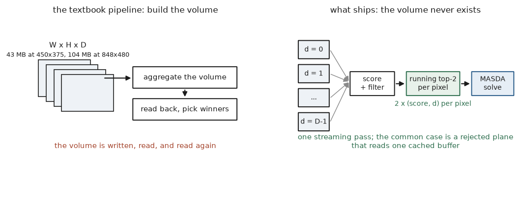
The insert’s common case is a rejection that reads one cached plane, so the whole stage is a single streaming pass over the scored planes. Removing the volume measured 1.9× end to end, and it is also what made the accuracy work possible: every parameter in the sweep was measured on a pipeline fast enough to iterate on.
Three structural properties fall out of this design and matter later:
- Rows are independent, because correspondences live on a rectified row. Each row is a separate MASDA instance.
- Disparity planes are independent until the top-2 insert, which is a per-pixel reduction.
- The aggregation needs whole constant-disparity planes. The recursive filter runs across the image at one disparity. This constraint decides the outcome of two separate experiments in what did not work, and it is the single most consequential property of the design.
2. Sub-pixel disparity: the largest accuracy result in the project
The solver picks a disparity from a discrete set, so its output is an integer. That forfeits up to half a pixel before any matching error, and fixing it is worth more than every other accuracy change in this post combined.
The fit is a parabola through the aggregated cost at the winning disparity and its two neighbours, with the vertex taken as the answer:
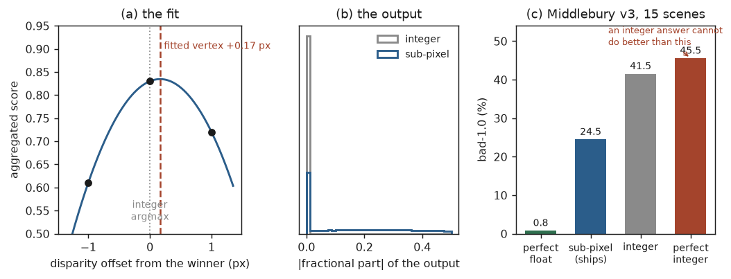
Panel (c) is the reason this matters and the reason it went unnoticed for a long time. A perfect integer disparity map scores 45.6% bad-1.0 on Middlebury v3 at quarter resolution. A perfect floating-point one scores 0.8%. The reason is the threshold. The benchmark allows one pixel of error at full resolution, and the matcher works at quarter resolution, so the allowance is a quarter of a pixel in the matcher’s own units. An integer answer can never land inside a quarter-pixel window, no matter how correct it is. The matcher’s own integer output measured 41.5%, which is close to that 45.6% ceiling: the matching was already good, and the output format was throwing it away.
With the fit: 41.5% → 24.5%, at coverage that does not move — 17 points. The fit changes values, never decisions.
The estimator matters as much as having one. Write \(c_0\) for the score at the winning disparity and \(c_{-1}, c_{+1}\) for its two neighbours. Fitting a parabola through the three and taking its vertex gives an offset
\[\delta \;=\; \frac{1}{2}\cdot\frac{c_{+1} - c_{-1}}{2c_0 - c_{-1} - c_{+1}}\]and the answer is \(d + \delta\), clamped to \(|\delta| \le \tfrac{1}{2}\). A parabola is the wrong shape for this cost. The graded score blends Census with a truncated absolute difference, which is piecewise linear, so the surface around the winner is locally a V rather than a bowl. Fitting two straight lines of equal and opposite slope instead — the equiangular estimator, the standard one for a V — changes only the denominator:
\[\delta \;=\; \frac{1}{2}\cdot\frac{c_{+1} - c_{-1}}{c_0 - \min(c_{-1},\, c_{+1})}\]Same three samples, same one line of code, no extra memory:
| estimator | bad-1.0 | coverage |
|---|---|---|
| parabola | 25.18 | 79.6% |
| equiangular | 24.47 | 79.6% |
equiangular, Census only (--ad 0) |
23.75 | 79.8% |
0.71 points for one line. The third row says the absolute-difference term still costs 0.72 even with the right estimator, so this is not purely an estimator mismatch — fitting on the Census term while selecting on the graded cost would collect the rest, at the price of a second filtered plane. Not built.
Two implementation details matter enough to describe.
Getting the neighbours back. The whole point of never building the volume is that the filtered cost volume does not exist, so the two costs the fit needs are gone by the time the winner is known. The cost stage now retains a three-wide window around each pixel’s running best — when a new best is set, the previous plane’s value is its left neighbour, and the next plane’s value is its right. That only works if the disparity planes arrive in order within a thread, which means the cost stage hands each worker a contiguous range of disparities instead of stealing single planes. Sizing those ranges by work rather than by plane count matters, because a plane’s cost is proportional to its valid width \(W - 6 - d\) and shrinks as \(d\) grows; equal plane counts would leave the low-\(d\) worker holding the most.
It costs 1.30× on the CPU. The three-wide window and the coarser work quantum both land on the cost stage. The first version cost 1.53×, and I fixed the wrong half of it first. Double-buffering removed the extra store and barely changed the wall clock, because the store was never the constraint. The chunked scheduler was. 16-plane chunks at \(D=60\) is four chunks for six threads, so two threads got nothing and occupancy fell from 5.3 of 6 cores to 3.7. That is worth more than the arithmetic it saved.
3. Measuring it: the benchmark had to change first
For most of this project the accuracy number came from eight Middlebury 2003/2005 scenes at 450×375, scored at native resolution. That benchmark is structurally incapable of seeing the sub-pixel result: at a one-pixel threshold on the native grid, integer output costs almost nothing. Sub-pixel disparity measured as slightly harmful there, was recorded as a negative, and sat disabled.
Middlebury v3 is where the field publishes, and its rules differ in a way that matters: the evaluation is always at full resolution, and it upsamples your result to get there. Disparity scales with resolution, so a quarter-resolution result has its disparities multiplied by four and its errors with them.
That trap is worth stating precisely, because the first evaluator I wrote fell into it. Scoring a quarter-resolution result against quarter-resolution ground truth at bad-1.0 gives 13.0% where the leaderboard says 37.3% for the same data. That is 2.9× too good, and it looks entirely plausible. What caught it was scoring Middlebury’s own published SGM output, which ships with the dataset and has a known row on the public table. An evaluator that cannot reproduce a known result is not evidence about anything. Mine now reproduces it to 37.33 against 37.3 and refuses to run if it stops.
The metric definitions are transcribed from the benchmark’s own evaldisp.cpp rather
than reimplemented, including two details that change the answer: the maximum disparity
for clipping comes from the result’s calibration while the integer-rounding flag
comes from the ground truth’s, and bad counts wrong pixels over all masked pixels
including the ones the matcher left empty. That last one means bad is not an error
rate over answered pixels until you divide by coverage.
4. What the matcher produces
All fifteen v3 scenes run, including the two with disparity ranges of 160 and 190. These are the eight 2003/2005 scenes, at their native resolution, so the disparity maps are directly comparable with the ground truth beside them. Black is “no answer” — either no ground truth, or the margin gate declining to commit:
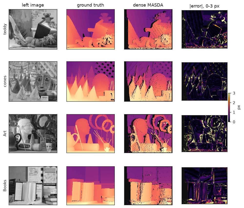
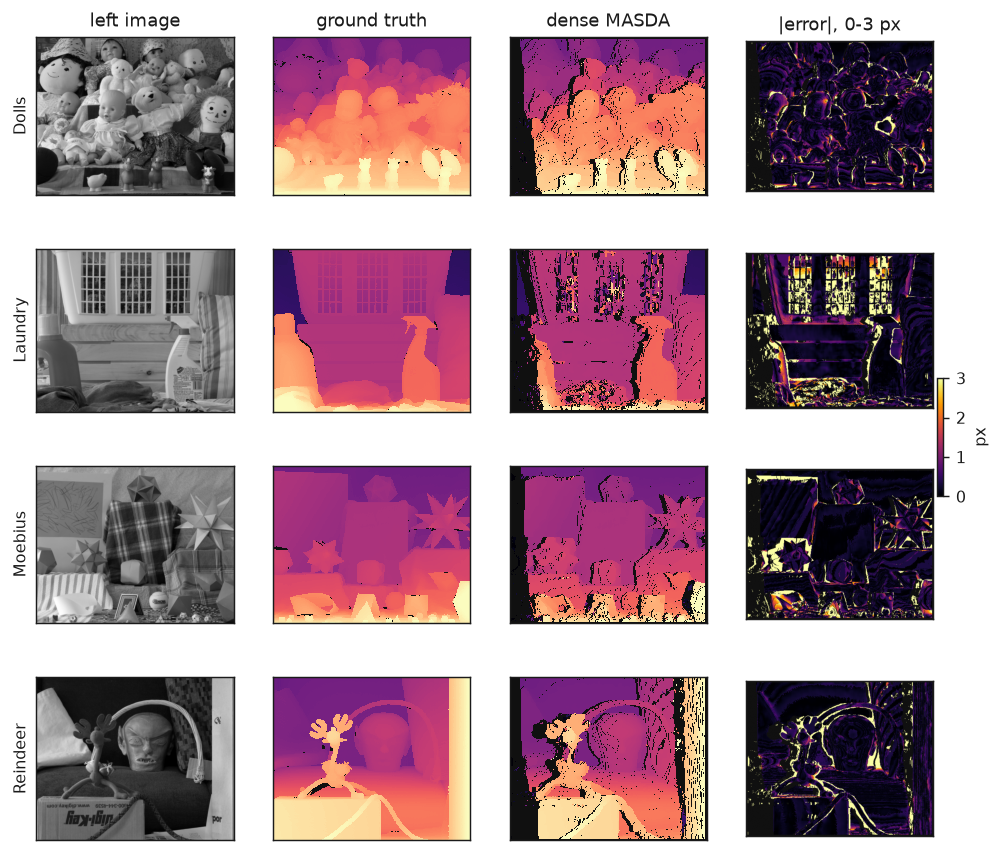
The error column is the interesting one. The residual error is at depth discontinuities and in repetitive texture, which is where Part 1’s ambiguity analysis predicted every matcher loses — including the exact assignment solver. The error budget measures exactly how much of the total error lives near discontinuities, because it turns out to decide whether a whole family of improvements is worth building.
5. The precision–coverage curve, and reading it against SGM
A matcher with a confidence gate does not have an accuracy. It has a curve, and the gate picks a point on it. Sweeping the margin gate across the fifteen v3 scenes:
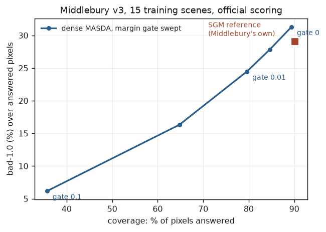
This is the only fair way to compare against a matcher that answers a different number of pixels. Read at matched coverage, SGM is ahead. Read at the shipping gate, this matcher has the lower error rate but answers ten points fewer pixels. Both readings describe the same picture: SGM’s curve sits below this one over the range where they overlap.
That is a different conclusion from the one the older eight-scene benchmark supports, where dense MASDA measures 9.8% bad-1.0 against OpenCV SGM’s 10.9%. Both numbers are real. The 2003/2005 scenes at native resolution are an easier problem scored at a looser tolerance, and the two benchmarks disagree about the ordering. When they disagree I take the harder one, but the older number is not wrong — it is answering a different question.
Where the coverage goes is worth knowing, because it is not lost:
| sink | coverage cost |
|---|---|
| the margin gate | 11.1 points |
| contention in the one-to-one decode | 0.2 points |
One property of the margin bounds how far it can be trusted, and it is not visible on a benchmark. Best-minus-second is only defined over the candidates actually searched. Where the true disparity is outside the search range, or its match lies off the edge of the other image, the best candidate has no real competitor and the margin is therefore large. On the camera this is not hypothetical: raising the gate to 0.05 on a scene whose near floor sat outside the search range removed a fifth of the wrong points and four fifths of the right ones. A confidence that reads only the cost curve cannot see the case where the answer was never on the curve.
98% of the coverage cost is the gate, which is a chosen position on the curve. I built the fix for the other 0.2 — when a pixel’s best candidate points at a right pixel some other pixel already claimed, retry its second candidate instead of dropping the pixel — and measured coverage 80.1% → 80.3% for error 26.0% → 26.3%. It pays for what it recovers. Reverted.
6. Where a pixel is actually lost
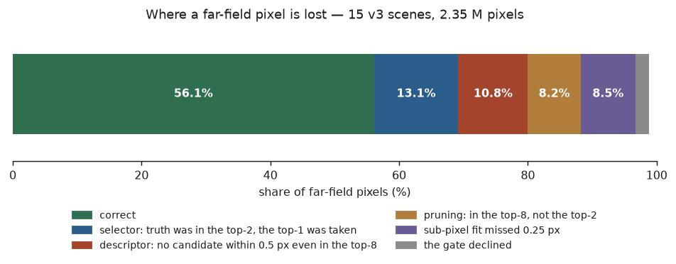
A single error rate says how often the matcher is wrong, not which component was wrong. Dumping the aggregated cost volume and asking where the true disparity ranks splits it. Over the 2.35 million far-field pixels — those nowhere near a depth discontinuity, which carry 71% of all error:
| a candidate within 0.5 px of the truth | top-1 | top-2 | top-4 | top-8 |
|---|---|---|---|---|
| far field | 67.9% | 81.0% | 85.8% | 89.2% |
| near a discontinuity | 58.8% | 75.7% | 84.6% | 90.1% |
Half a pixel is the threshold that matters, because a candidate that close is the nearest integer to the truth and the sub-pixel fit can still reach the answer. A candidate a full pixel away cannot be refined into a correct one.
Reading the bill:
- The descriptor is the largest single item. 10.8% of far-field pixels have no candidate within half a pixel anywhere in the top eight — unreachable by any solver on this cost volume — and 19.0% are unreachable without keeping more than two candidates.
- 13.1% is the selector’s. The truth is in the top-2 and the top-1 was taken. That is the one component with a clear mandate and no mechanism currently collecting it: the ablation shows that neither winner-take-all nor message passing gets it.
- 8.5% is the fit, on pixels whose integer was already right.
One methodological note, because it changed the answer. Run on Teddy alone, this table says the fit is dominant and the descriptor is nearly free — Teddy’s cost is much better than average, 92.8% top-1 in the far field against 67.9% pooled. The fifteen-scene number inverts the ordering. One scene is not a benchmark, and this is the cleanest demonstration of that in the project.
7. What the parameters are worth
Every parameter in the matcher, swept on the fifteen v3 scenes at the shipping configuration. Some of these had never been measured, and one of them had never been measured at all despite carrying a comment that implied it had.
Aggregation reach \(\sigma_s\) — was set past its optimum. The comment beside it recorded a sweep of the range parameter \(\sigma_r\), and \(\sigma_s\) had simply inherited a value:
| \(\sigma_s\) | 6 | 8 (now) | 10 | 12 (was) | 20 |
|---|---|---|---|---|---|
| bad-1.0 | 24.98 | 25.18 | 25.61 | 26.17 | 28.32 |
| coverage | 79.9% | 79.6% | 79.3% | 78.9% | 77.8% |
(This sweep and the two below predate the equiangular estimator, so their absolute values sit 0.7 above the current operating point. The shapes are what they are for.)
Better on both axes at 6–8 than at 12, and free: the filter is an IIR whose cost does not depend on \(\sigma\). Now 8. This is the cheapest 0.9 points in the project and it was sitting there because a comment about a neighbouring parameter made the value look considered.
The graded cost interacts with the sub-pixel fit, and the benchmarks disagree. The truncated absolute difference blended into the Census score was measured at 10.3% → 9.7% when it was added:
--ad |
0 | 0.08 | 0.15 (ships) | 0.25 |
|---|---|---|---|---|
| bad-1.0 (v3) | 24.42 | 24.68 | 25.18 | 26.13 |
On v3 it now measures the other way — and the entire effect is the fit. With sub-pixel
disabled, ad 0 gives 42.00 and ad 0.15 gives 42.04, which is nothing. The truncated
difference saturates and is piecewise linear, so blending it into the cost changes the
shape near the minimum. An argmax does not care about shape; a parabola through three
samples cares about very little else. On the older eight-scene benchmark, scored at
native resolution where the fit’s quality is invisible, the graded cost still helps —
9.8% against 10.3%, and better coverage. It stays on, because that is the resolution
and tolerance the camera actually operates at, and the interaction is recorded rather
than tuned away. The change that would win on both is to fit on the Census term alone
while still selecting on the graded cost, which costs a second filtered plane.
\(\lambda\) and \(\gamma\) do nothing where they are set. These are MASDA’s clutter and misdetection costs — the price of leaving a left pixel unmatched and a right pixel unclaimed:
| \(\lambda = \gamma\) | −0.4 | −0.1 (ships) | +0.3 |
|---|---|---|---|
| bad-1.0 | 25.18 | 25.18 | 22.02 |
| coverage | 79.6% | 79.6% | 73.4% |
Below zero they are not merely flat — a factor of four in magnitude produces a byte-identical disparity map. They sit far below the score distribution, so the rejection they implement almost never fires. Above zero they work — and what they do is trade coverage for precision at roughly the same exchange rate as the margin gate, which is to say they are a second gate rather than a second mechanism.
Descriptor size trades, it does not improve. The obvious response to a 10.8%
descriptor bill is a bigger descriptor — the Census window is a template and 9×7 is 62
bits, which still fits a uint64. Before touching fifteen border literals in the cost
loops and the CUDA census kernel, the direction was priced on the axis already wired.
--csct is the same Census at 24 bits instead of 48:
| bad-1.0 | coverage | |
|---|---|---|
| 7×7 Census, 48 bit | 25.18 | 79.6% |
| centre-symmetric, 24 bit | 24.68 | 75.9% |
Halving the descriptor lowers the error rate by 0.5 and costs 3.7 points of coverage. That is the same precision–coverage trade every other knob offers — not a better or worse descriptor, a differently-gated one. If 24 fewer bits only slides along the curve, 14 more will too, so 9×7 is not worth building.
Which sharpens what that 10.8% is: not a bits problem. More of the same descriptor will not collect it. It is a limit of Census-plus-truncated-difference as a similarity measure on weakly textured and repetitive surfaces, and changing that means changing the similarity function itself.
And one flag does nothing at all. --agg, the aggregation radius, produces
identical output at 3, 7 and its default, because the recursive filter ignores it. It
still exists as a flag because an older box-filter path used it. Stated here so that
nobody sweeps it and wonders why nothing changes.
8. The ablation: the message passing is not what makes this work
The matcher is named after an inference algorithm, so the obvious question is what that inference contributes. Disabling the message passing leaves everything else in place: the candidate set, the one-to-one decode, the margin and the gate. The decision is then made by score alone. That is winner-take-all with a uniqueness constraint on top:
| iterations | K = 2 (ships) | K = 8 | ||
|---|---|---|---|---|
| bad-1.0 | coverage | bad-1.0 | coverage | |
| 0 — winner-take-all (ships) | 25.18 | 79.6% | 24.41 | 79.8% |
| 1 | 26.13 | 79.6% | — | — |
| 2 | 26.04 | 80.1% | 25.58 | 80.6% |
| 4 | 26.19 | 80.2% | 25.78 | 81.0% |
The message passing buys coverage and pays for it in precision, at about the same exchange rate as the gate and \(\lambda/\gamma\). It is a third knob along the same curve. And it is not free: on the TX2 the solve is 13.0 ms without it against 25.5 ms with it, so roughly twelve milliseconds of CPU at the camera’s resolution.
Getting this measurement right required fixing the ablation first. With no messages the max-sum belief \(\beta + \rho - s\) degenerates to minus the score, so the solver picked the worst candidate and the configuration read 67.3% — which looks exactly like proof that message passing is worth forty points. It is not an ablation, it is an inverted objective, and it would have been an easy number to publish.
What this does not say is that MASDA is doing nothing. The parts that survive the ablation are the parts that distinguish this from a block matcher: the one-to-one constraint, which SGM does not have at all and needs a left-right consistency check added afterwards to approximate, and the margin, which is what a downstream consumer gates on. Both are present in every row of that table. What is in question is the loopy belief propagation on top of a two-candidate set, which is the case where it has the least to decide. The sparse matcher’s advantage in Part 1 was measured with many candidates on deliberately ambiguous projected-dot texture, and temporal association — where the candidate set is genuinely large and two-dimensional — has not been tested. Message passing is off by default in the dense path and one flag away.
The camera adds a detail the benchmark cannot show. Take a live scene where part of the floor falls outside the search range, so those pixels have no correct answer available at all. Raising the iteration count moves coverage from 88.3% to 90.0%. It also moves the number of points sitting on a demonstrably false surface from 242 to 473, and the extra ones are concentrated in the strip where the correct match lies off the edge of the right image. The extra coverage is partly coverage of pixels that cannot be answered: message passing propagates support along the row, and where no correct answer exists it propagates the wrong one and raises its confidence. A one-to-one constraint does not reject an occluded pixel when the true partner is outside the image, because there is no competitor for it to lose to.
9. What did not work, and why
Four families of improvement were measured and declined. Each was priced before it was built, which is the only reason the list is short.
Restricting the disparity range — 5.2× on paper, 1.9× in practice. Every fast published CPU matcher avoids the exhaustive sweep: ELAS triangulates support points, PatchMatch propagates hypotheses, rSGM subsamples. The ceiling is real — if each 16×16 tile knew which disparities its pixels needed, it would compute 19.2% of the sweep. Three things consume that saving:
- Per-pixel restriction is illegal here. The filter aggregates over a plane, so a plane must hold one constant disparity. Restriction has to be per-tile, so that every pixel in a tile sweeps the same set.
- The best available predictor is not accurate enough. A half-resolution pass predicts tile ranges at 20.9% of the sweep — essentially at the oracle’s cost — but with 90.7% recall, meaning one true disparity in eleven falls outside its tile’s band. Reaching a usable recall costs most of the saving.
- The aggregation needs its input. A tile can only skip a plane if it also skips it for the pixels the filter reads, and the filter reaches ~16 px. A 16×16 tile wanting one plane costs a 48×48 patch of it. That takes 26.3% to 53.8%.
Intrinsic curves deserve a separate mention because they reproduce their paper exactly and still do not help. The construction admits 13.9% of the disparity range per pixel — an 86% reduction, right at the published claim. But the admitted disparities of neighbouring pixels do not agree: the union over even a 4×4 tile is 43.6% of the range. A reduction that is per-pixel and spatially incoherent is unusable by a matcher that aggregates over planes, and usable by one that scores candidates individually — which is what that paper’s own SGM does.
Better edge-aware support — the target is real, the mechanism is not. Pixels within 8 px of a depth discontinuity are 18.3% of the image and carry 28.6% of all error, at 57.1% against a 32.0% far-field rate. That is a 4.6-point target. But two independent knobs that should move it do not: a fourfold range of the filter’s edge sensitivity leaves near-edge error at 57.1–57.8%, and handing the solver the entire disparity range instead of two candidates leaves it at 56.4%. What remains is half-occlusion — beside a foreground edge, part of the support has no correspondence in the other image at all, and no weighting scheme fixes neighbours that are not visible. The aggregation here is already edge-aware; making it more or less so does not touch the pixels it was supposed to help.
A second search band around the coarse level’s runner-up. MASDA exports its second-best candidate, and at thin structures the runner-up is often the surface the best candidate missed. Measured: worse everywhere. Where the coarse level is ambiguous its runner-up is the wrong period of a repetitive texture, and a band around it hands the fine solver a wrong surface it can aggregate into a confident answer.
A strict per-pixel band-membership test at insert time — the principled version of a masked search. Measured a full point worse. The row-interval slack admits candidates a pixel’s own band would exclude, and they help.
The last two point the same way as Part 1’s central result: exact per-row assignment is no more precise than MASDA on identical candidates, so the inference is not what bounds the outcome. The candidate set is. What you offer the solver matters more than how cleverly you restrict it, and both of these experiments restricted it cleverly.
10. Where this leaves the CPU implementation
At the camera’s 848×480 the CPU matcher is a 5 Hz matcher, and the solve — the part that is MASDA — is memory-bound rather than arithmetic-bound. Two structural properties say where it goes next, and neither is a CPU optimisation. Disparity planes are independent, rows are independent, and the solver is two strided reductions. That is a description of a CUDA kernel, and the TX2’s GPU sits at load zero through everything above.
Part 3 is that port: the image plane moves to the GPU, the CPU keeps the graph, and the matcher runs at 31.7 ms per frame at 848×480, bit-identical to this implementation on all eight ground-truth scenes.
The methodological part is worth keeping even if the matcher were thrown away. Three rules, each paid for:
- The desktop is not a proxy for the target, in either direction. int16 arithmetic was neutral on the desktop and worth 20% on the Jetson; a 24-bit descriptor was worthless on the desktop and worth 10% on the Jetson; a coarse-to-fine mask was worth 1.24× on the desktop and flat on the Jetson.
- The benchmark decides what you can see. Sub-pixel disparity was a recorded negative for months because the benchmark in use could not resolve it.
- Check that a default change is live before measuring it — twice over. A header
was listed as a prerequisite in one build rule and not the other, so a header-only
change relinked nothing,
makeprinted success, and a fifteen-scene benchmark measured the old value and reported it as the new one. Then both benchmark harnesses turned out to pass--iterswith values of their own, silently overriding the binary’s default — so “the default configuration” had for weeks meant the harness’s opinion, and a default change read as no change whatsoever. Both were caught by a number coming back exactly equal to a figure that should have moved. An unchanged measurement is a weaker signal than an error, and a slightly different one would have been believed.
The matcher is de_dense.cpp, plain C++14 with no dependencies. Every figure in this
post is regenerated from the shipping binary by one script, and every number by one
benchmark command against Middlebury ground truth.
References
Full citations with DOIs, and every term this post uses, are in the series glossary.
- Geiger, Roser, Urtasun, Efficient Large-Scale Stereo Matching (ELAS), ACCV 2010 — support points and a triangulated prior; the canonical “don’t sweep” CPU matcher.
- Bleyer, Rhemann, Rother, PatchMatch Stereo, BMVC 2011 — hypothesis propagation instead of a sweep, and slanted support windows.
- Spangenberg et al., Large Scale Semi-Global Matching on the CPU, IV 2014.
- Ruf et al., ReS2tAC, Sensors 21(11), 2021 — the disparity-in-the-lanes formulation, and the embedded CUDA baseline Part 3 measures against.
- Nover, Achar, Goldman, ESPReSSo, 3DV 2018 — edge-aware aggregation under shared plane hypotheses; the one remaining candidate for range restriction that produces tile-constant hypotheses by construction.
- Shahbazi et al., Revisiting intrinsic curves for efficient dense stereo matching, ISPRS 2016 — the per-pixel range reduction measured in what did not work.